HTC calculations in PanSolidification
- Purpose: Users have learned to obtain the crack susceptibility index (CSI) value of a single alloy under certain solidification conditions in Solidification simulation of an Al-Cu-Mg alloy for hot cracking susceptibility index prediction. In this example, users will learn to use High Throughput Calculation (HTC) calculations to obtain a susceptibility index map in Al-Cu-Mg ternary system
- Module: PanSolidification
- Database: PanAl2020_TH+MB.pdb; Al_Alloys.sdb
Calculation Method:
- Create a workspace and select the PanSolidification module. Save the workspace in a user assigned folder different from the default workspace. The HTC calculation results will be saved automatically under this folder. (Detailed description also in Pandat User’s Guide 2.1)
- Load PDB file PanAl_TH+MB.pdb through menu Database->Load TDB or PDB (Encrypted TDB) or by click icon
 , and select the elements: Al, Cu, Mg.
 - Load SDB file sdb through menu PanSolidification->Load SDB or by click icon
 , select the available alloys: Al alloys.
 - Start HTC function through menu Batch Calc->High Throughput Calculation (HTC).
- Choose calculation type from the drop-down list of HTC pop-up window and select “pan_solidification” as shown in Figure 1.
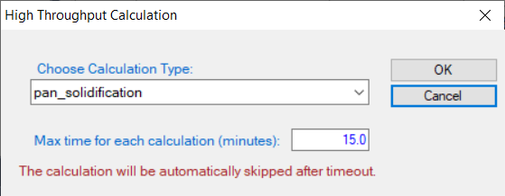
Figure 1. Dialog to choose calculation type of HTC in PanSolidification
- Define the compositional space for HTC simulation. The composition range is set to 0-5 wt.% Cu and 0-5 wt.% Mg, and mouse right click on the composition field of Al to set as the remaining composition, which is shown as -1 in all the composition field of Al, as shown in Figure 2.
- Define the solidification conditions for HTC simulation. The same solidification conditions with cooling rate of 20 K/s and Temperature gradient is set as 10-3 °C/μm, as shown in Figure 2.
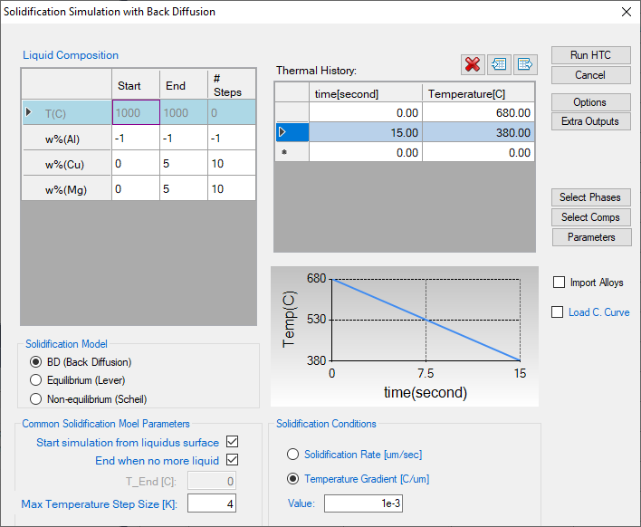
Figure 2. Dialog to setup compositional space and solidification conditions for PanSolidification HTC
- Set “Extra Outputs table”. Click the “Extra Outputs” in Figure 2. The following extra output is defined as shown in Figure 3: time; T – temperature; w(*) – alloy composition; fs – solid phase fraction; sqrt(fs) – the square root value of the solid phase fraction; and -T//sqrt(fs) – the CSI index. Then click OK.
- Set “Extra Outputs graph”. Using the procedure described in Solidification simulation of an Al-Cu-Mg alloy for hot cracking susceptibility index prediction, click the icon “Graph” in “Set extra output”, set sqrt(fs) as X axis and -T//sqrt(fs) as Y axis. Then click OK.
- Click “Run HTC” button to perform HTC simulations.
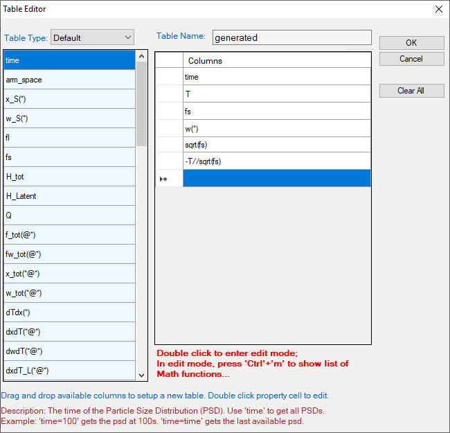
Figure 3. Define properties in the extra output table
Post Calculation Operation:
- After all calculations have been finished, analyze the results through menu Batch Calc->Result Analysis. User can then analyze the results of the selected HTC calculation by opening the corresponding workspace as shown in Figure 4.
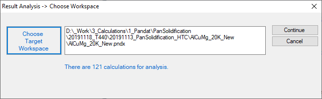
Figure 4. “Result Analysis” popup dialog to choose target workspace
- Define the criteria of the properties as filters for result analysis. As shown in the following Figure 5, analysis the “generated table”, set the condition to find the CSI for each alloy composition, i.e., CSI = MAX(-T//sqrt(fs)) at sqrt(fs)< 0.99.
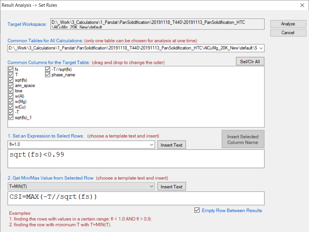
Figure 5. Criteria for Cracking Susceptibility Index setting from solidification results analysis
- After results analysis, a table which list CSI = MAX(-T//sqrt(fs)) for each alloy composition is generated as shown in Figure 6.
- Select w%(Cu) as X-axis, press Ctrl then select w%(Mg) and (-T//sqrt(fs)) as Y-axis and Z-axis, respectively, click
 on the tool bar to generate Figure 7 which shows the crack susceptibility map for Al-Cu-Mg alloys with cooling rate of 20 K/s.
 - The simulated result is comparable with the experimental results shown in Figure 8.
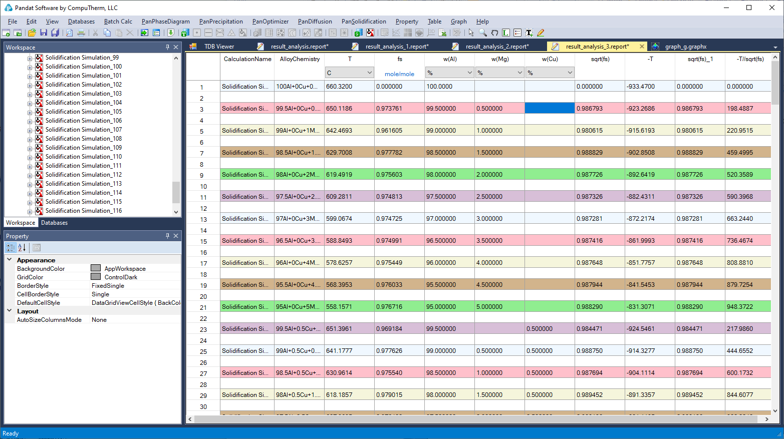
Figure 6. A table which lists the CSI = MAX(-T//sqrt(fs)) for each alloy composition is generated after the results analysis
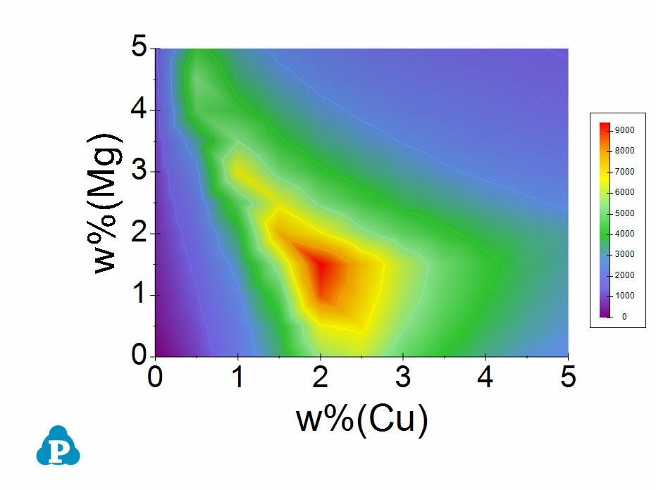
Figure 7. Al-Cu-Mg crack susceptibility map with cooling rate of 20 K/s
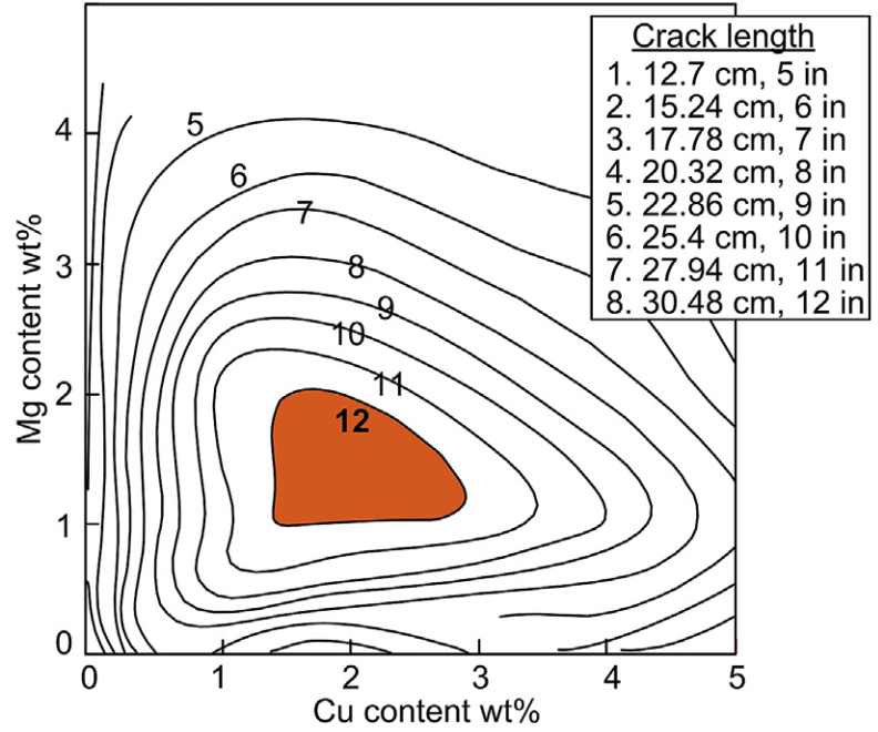
Figure 8. Experimental crack susceptibility test results