7
2 Get Started
Pandat
TM
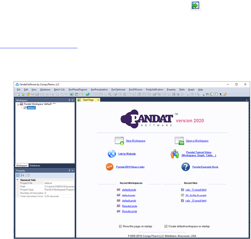
starts with the following start page as shown in Figure 2.1. The user
can open the start page at any time by clicking the icon on the toolbar. On
the start page, there are shortcuts which allow users to create a new
workspace and open an existing workspace, link to CompuTherm’s webpage
(www.computherm.com) for recent updates and for comments and discussions
from Pandat
TM
users. It also lists the most recent workspaces and files the user
has created, so that user can reopen them easily.
Figure 2.1 The start page of Pandat
TM
software
2.1 Workspace
The workspace provides a space for user to perform Pandat
TM
calculations and
organize the calculated results. It must be created before any Pandat
TM
calculation is carried out.
8
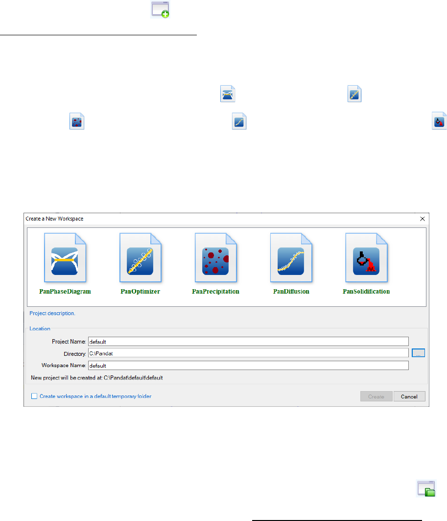
User can create a new workspace by clicking on the “New a Workspace” link on
the start page, or the icon on the toolbar, or go through the menus
(File → Create a New Workspace). A new window will pop out as is shown in
Figure 2.2. User can define the name of the workspace and select a working
directory to put the workspace. User can then select the module from the five
icons: Phase diagram calculation ( ), Optimization ( ), Precipitation
simulation ( ), Diffusion simulation ( ) or Solidification simulation ( ).
User can also give a “Project Name” for the calculations to be performed. User
may choose to create a default workspace with default project name simply by
clicking the “Create” button or double click the selected module.
Figure 2.2 Create a new workspace dialog
After using Pandat
TM
, user will be given an opportunity to save the workspace
that the user has created. The user can open a saved workspace next time by
clicking on the “Open a Workspace” link on the start page, or the icon on
the toolbar, or going through the menus (File → Open → Workspace). For
some most recent workspaces and files, the shortcuts listed on the start page
allow the user to open them directly.
In Pandat
TM
, only one workspace is allowed. When creating a new workspace,
the user will be asked if the current workspace needs to be saved. Think twice

9
before clicking the “Create” button. The old workspace will be lost if it is not
saved when a new workspace is created.
2.2 Project
In the Pandat
TM
, a workspace may contain many projects of different types. For
example, a user creates a project for PanPhaseDiagram module which
contains all calculations for phase diagrams. User can then create a new
project of precipitation simulation in the same workspace using menus (File →
Add a New Project). In this case, the workspace name and the working
directory cannot be changed, but the user needs to give a new project name.
The database file, table, graph and other data associated with one project can
be viewed in individual tabs in the Display window.
When more than one project are created in one workspace, only one project will
be activated at one time, and only those functions and toolbar icons associated
with the activated project are available to the user at the time.
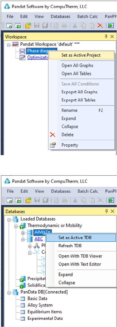
The name of the activated project will be highlighted as blue and be underlined.
To select a project as the activated project, right click the mouse on the project
name in the explore window and choose “Set as Active Project” in the popup
dialog as shown in Figure 2.3.
When switching between projects, the user may also need to swtich between
different databases so that the right database is used for the calculation. In the
Databases view dialog in explore window, all the loaded databses are listed and
the name of currently activated database is also highlighted with blue and be
underlined. To activate another database, right click the mouse on the
database name and choose “Set as Activate TDB” as also shown in Figure 2.4.
Inside one project, the user may also load several databases and carry out
10
different calculations of the same type. The user need to make sure that the
correct database is activated when performing a calculation.
Figure 2.3 Set an active project
Figure 2.4 Set an active database
11
2.3 Graph
In each project, the calculated results are presented in two different formats:
Graph and Table. Graph is one of the most important parts in Pandat
TM
interface. A typical Pandat
TM
graph includes at least three elements: a set of X
and Y coordinate axes, one or more data plots and associated text and drawing
objects. Each graph can have one or more data plots and these data plots can
be configured individually. Each data plot corresponds to a data set which can
be either calculated results or experiment data.
The graph is plotted in the main display window with Pandat
TM
logo. The
Property window defines the properties for all the elements in the graph in
detail. When a typical element is selected, the property of this element will be
displayed in the Property window and the user may modify the graph through
the Property window.
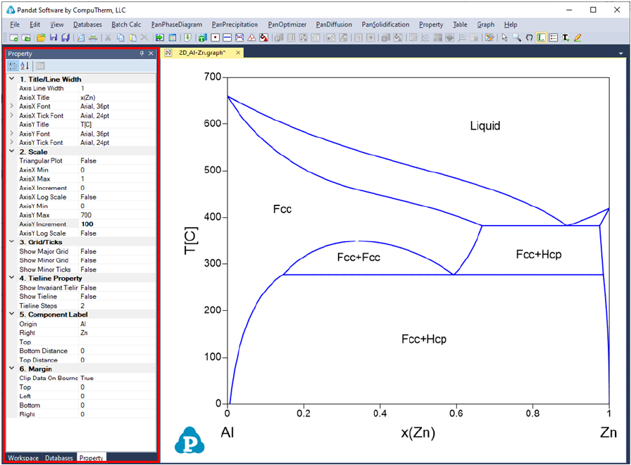
2.3.1 Property
The overall property of a graph consists of six categories: Title/Line Width,
Scale, Grid/Ticks, Tieline Property, Component Label and Margin, as
shown in the red box area in Figure 2.5. All six categories will be shown in
Property window when the whole graph is selected. The Title property defines
the axis line width, the title, title font size and tick font size for both X axis and
Y axis. The Scale property defines the minimum and maximum values,
increment and Log scale status for both X and Y axises and a flag of Ternary
Plot. If this flag is set as “True”, the figure is plotted as Gibbs triangle for a
normal isothermal section and only the increments are also shown in the Scale
property. If the flag is set as “False”, a Cartesian coordinate figure will be
plotted. The Grid/Ticks property defines whether to show grids on the graph or
ticks on the axis. The Tieline Property defines whether to show the tie-lines and
the density of the tie-lines. The Component label defines the labels on the
origin, right corner and Top corner of the graph. The Margin property defines
the position of the plot in the Main display window.
12
Figure 2.5 Graph property window
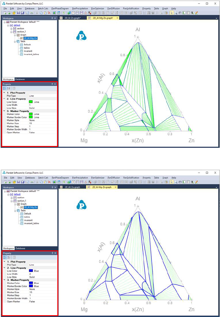
The other properties of the tie-lines, such as the color, the style, are defined by
individual property window associated with these tie-lines. These properties
can be modified when only the tie-lines on the Main Display window are
13
selected and highlighted as shown in
Figure 2.6. User can change the appearance of a set of lines belonging to the
same group by selecting this line (or a group lines) only. The properties for
such data plots, such as the line color, thickness, marker type, will show up in
the Property window for user to modify. The data points and lines selected will
be highlighted in the graph while the others will be grey. As shown in Figure
2.7, the phase boundary lines are selected as a group of lines to be modified in
this case. The properties of this group lines are defined in the Plot Property
window as “Blue, Solid, None marker” lines. All these properties can be
modified in the Property Window as framed by the red line in Figure 2.7. The
Line Property defines the property of the line and the Marker Property
defines the property of the point on the graph.
14
Figure 2.6 Tie-line property window
Figure 2.7 Plot property window
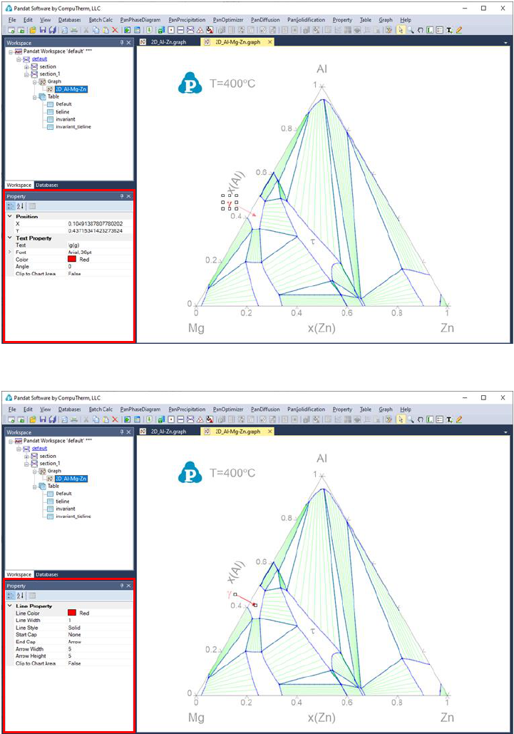
User can add texts and lines/arrows freely to the graph. The Text Property
defines the position, content, font size, color and rotating angle of the text, as
shown in the red box in Figure 2.8 when the text box is selected. The Line
16
2.3.2 Export a graph to other format
The user can output the Pandat graph to other popular formats such as emf,
bmp, jpg, png, gif and tif. The command is located on the menus: Graph →
Export, or right click the mouse on the graph and choose “Export” from the
popup menu.
2.3.3 Useful icons for Graph on Toolbar
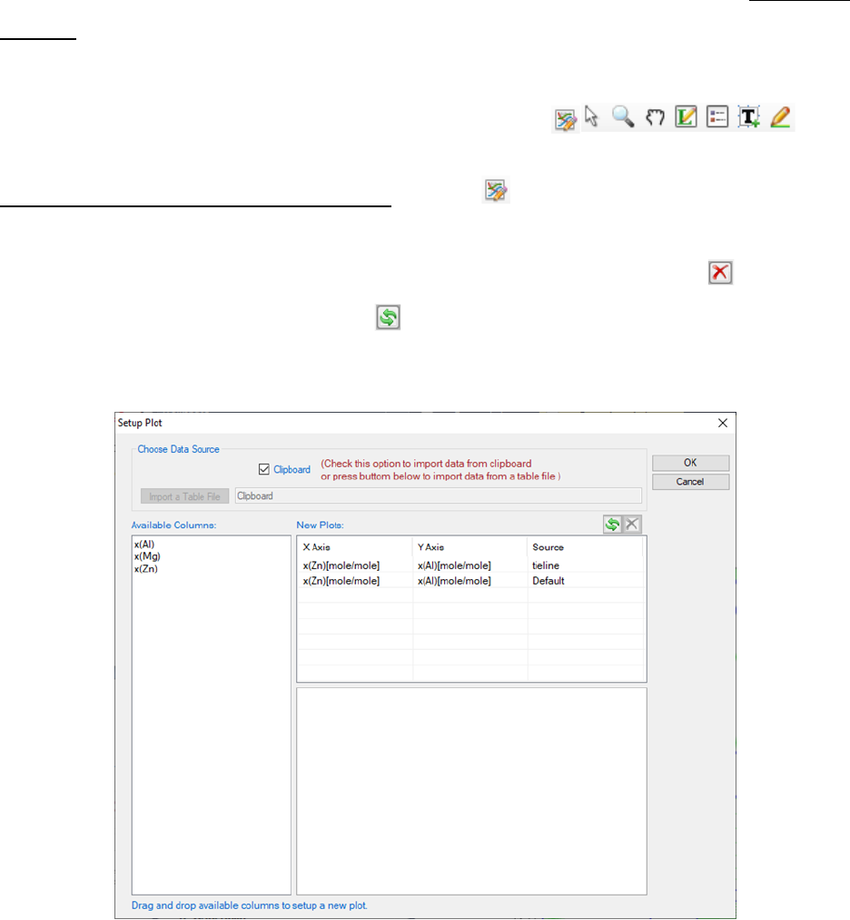
Edit Plots for the Current Graph button , allow the user to modify the
plots, such as add data plots with mouse drag and drop to set up x and y of the
new plot as shown in Figure 2.10, delete data plots using button , exchange
x and y of the plots using button . The available columns can be imported
from a file or from Clipboard if the check box in front is selected.
Figure 2.10 Set up data for X and Y for a plot
The table file to be imported can be Pandat
TM
table format or ASCII text format.
For a general Microsoft Excel table, the user can copy the selected columns in
17
the Excel file and check the Clipboard option, and then the column names will
show up in the “Available Columns” dialog for the user to select, which is also
shown in Figure 2.10. User can also copy the data from the table columns in
the Pandat
TM
calculation results.
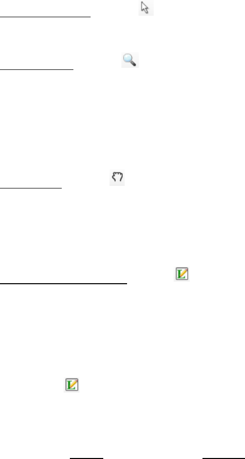
Select Objects button , allow the user to select drawing elements in a graph
such as line, arrow or text.
Zoom Mode button , use the Zoom mode to enlarge a small part of a graph.
Hold the left button of the mouse and move the mouse to select a rectangular
area on the graph to enlarge. The graph will zoom in to the selected area when
the left button of the mouse is released. Double click this button will bring the
zoom image back to the whole diagram again.
Pan Mode button , when this mode is on, put the cursor on the plot and roll
the mouse wheel to enlarge or shrink the graph, keeping the current center of
the graph unchanged. Hold the left button of the mouse on the graph and move
the mouse, the user can move the whole graph.
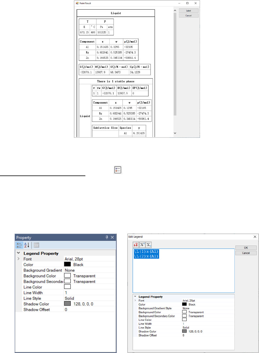
Label Phase Region button , label the graph with text. Pandat
TM
can not
only label the normal T-x or x-x phase diagrams from calculations, but also
label those user generated graphs using the table data from calculation, i.e., G-
x and μ-x diagrams. The user can modify the labeled text like normal text. If
the user holds the <Ctrl> key first and then click the mouse on the diagram
with the function, the program will do a point calculation at the
composition and temperature where the cursor locates. A new window will pop
out to show the calculated result in detail as shown in Figure 2.11. The user
can choose Label after reading or Cancel to close this window.
18
Figure 2.11 Point calculation result for the combination of the “Ctrl” key and
Labeling function
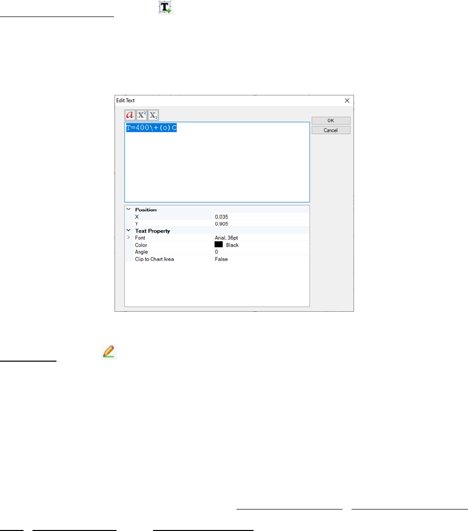
Add Legend for Graph button , add legend to the graph. The user can
modify the legend using the Property window, as shown in Figure 2.12(a).
Double click on the inserted legend will open a new Text Editor window as
shown in Figure 2.12(b), and the user can input complex text, such as symbol,
superscript and subscript in this windows.
(a) (b)
Figure 2.12 (a) Legend property window and (b) Legend editor window
19
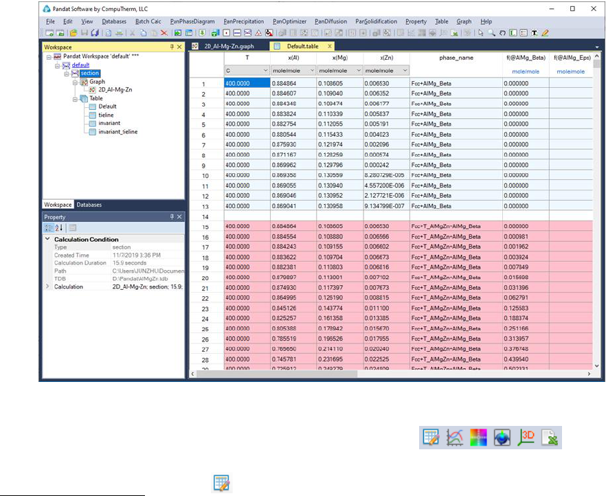
Add Text or Label button , add text to the graph. Change the text content,
size, color and rotating angle in the Property window. Double click on the text
also open the Text Editor window which allows user to input complex text in it
as shown in Figure 2.13.
Figure 2.13 Text editor window
Add Line button , add line with or without arrow to the graph. Change the
line or arrow width and color in the Property window. The default line has one
arrow at end of the line. User can set the start cap and end cap in the Line
Property window as shown in Figure 2.9.
2.4 Table
The menu of Pandat
TM
Table includes: Add a New Table, Import Table from
File, Create Graph, and Export to Excel. A typical table is shown as Figure
2.14. Each column of data is associated with a corresponding unit. The user
can change the unit of each column and observe the instant change of the
table values.
20
Figure 2.14 Table view of the calculation results in Pandat
TM
2.4.1 Useful icons for Table on Toolbar
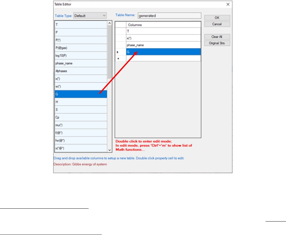
Add a New Table button , click this button or right click the mouse on the
Table node in the Explore window and select “Add a New Table”, a window of
Table Editor as shown in Figure 2.15 will pop out. User can create a new table
by dragging and dropping the available properties in the left dialog to the right
dialog as shown by the red arrow in Figure 2.15, and then click “OK” to
generate a new table with the selected properties.
21
Figure 2.15 Table Editor
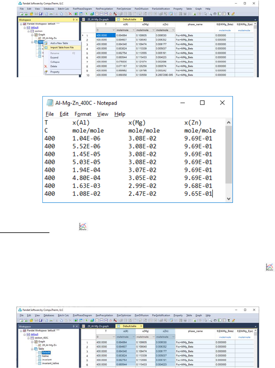
Import Table from File, User can import a customized table from an existing
file. This can be done by choosing the command located on the menus: Table
→ Import Table from File, or right click the mouse on the Table node and
choose “Import Table from File” from the popup menu as shown in Figure 2.16.
Pandat
TM
can read data files with “.dat” and “.txt” as default file extension
names. Figure 2.17 shows a typical data file for importing into Pandat
TM
.
Different columns are separated by Tabs. The first row defines the data name
for each column. The second row defines the unit for the data in each column
and the following rows define the data values. If the column names are the
same as those in the default table, the second row (the unit row) can be blank
and Pandat
TM
will use the same units as those in the default table.
22
Figure 2.16 Import a table from an existing file
Figure 2.17 A typical data file for importing
Create Graph button , create a new graph for the selected properties. Use
the <ctrl> key and the left button of the mouse to select multiple columns in
the table as shown in Figure 2.18. The first selected column will be the x and
the other columns will be the y’s for the new plots. After click on the
button, a graph will then be generated in the Pandat
TM
main display window as
shown in Figure 2.19.
Figure 2.18 Select data for creating a new graph
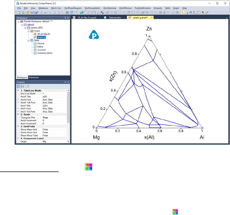
23
Figure 2.19 A new graph created from selected columns in the table
Create Color Map button , create a new color map graph for the selected
properties. Use the “ctrl” key and the left button of the mouse to select multiple
columns in the table as shown in Figure 2.20. The first selected column (x(Mg))
will be the x’s, the second column (x(Zn)) will be the y’s and the third column
(T) will be the z’s for the new plot. After click on the button, a color map
graph will then be generated in the Pandat
TM
main display window as shown in
Figure 2.21, where the liquidus temperatures are represented by different
colors.
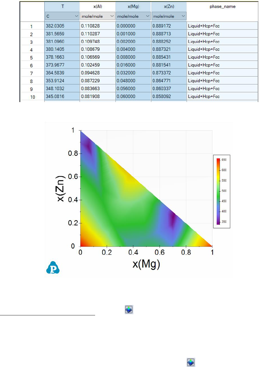
24
Figure 2.20 Select data to create a new color map graph
Figure 2.21 A new color map graph created from selected columns in the
isotherm table from the liquidus projection calculation
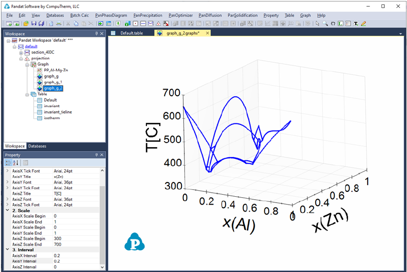
Create 3D Surface Graph button , create a new 3D surface graph for the
selected properties. Use the “ctrl” key and the left button of the mouse to select
multiple columns in the table as shown in Figure 2.20. The first selected
column will be the x’s, the second column will be the y’s and the third column
will be the z’s for the new plot. After click on the button, a 3D liquidus
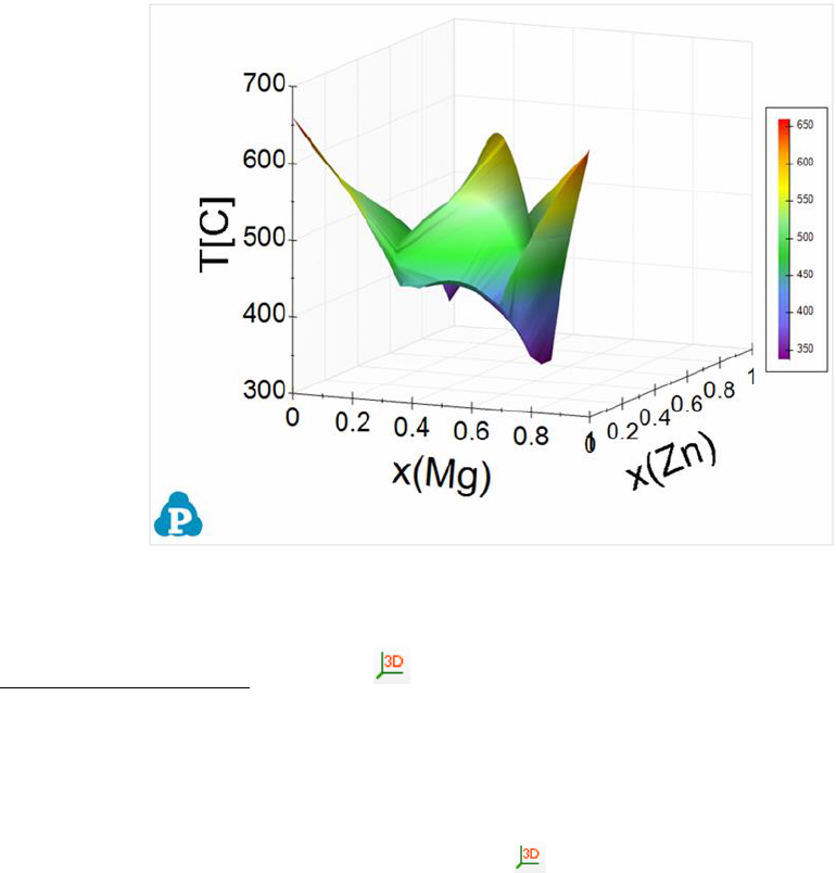
25
surface graph will then be generated in the Pandat
TM
main display window as
shown in Figure 2.22.
Figure 2.22 A new 3D liquidus surface graph created from selected columns in
the isotherm table from the liquidus projection calculation
Create 3D Graph button , create a new 3D graph for the selected
properties. Use the “ctrl” key and the left button of the mouse to select multiple
columns in the table as shown in Figure 2.20. The first selected column will be
the x’s, the second column will be the y’s and the third column will be the z’s
for the new plot. After click on the button, a 3D graph will then be
generated in the Pandat
TM
main display window as shown in Figure 2.23
representing the monovariant lines of the liquidus projection.
26
Figure 2.23 A new 3D graph created from selected columns in the table
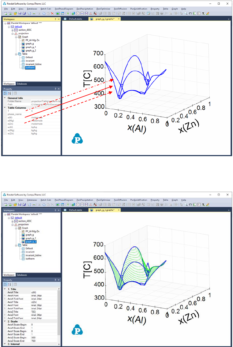
User can add more plots to the 3D graph. First click on the table containing the
data, i.e. isotherm data in Figure 2.24, and the property window will show the
column names in this table. Then select the column “x(Al)” as x-axis in the
property window, drag and drop it to the graph; then hold the “Ctrl” key and
select the second column “x(Zn)” as y-axis, drag and drop it to the graph; and
then hold the “Shift” key, select the third column “T”, drag and drop it to the
graph. The new plot of the data will be added to the original 3D graph shown as
Figure 2.25.
27
Figure 2.24 Add a plot to a 3D graph using selected columns in the table as
follows: (1) Solid arrow: drag and drop, (2) Dash arrow: drag and drop with the
“Ctrl” key held, (3) Dash dot arrow: drag and drop with the “Shift” key held
Figure 2.25 3D graph with multiple plots

28
Export to Excel button , allow user to export the table of interest (It must
be available in main display windows to activate the function button) directly to
a Microsoft Excel file. Excel must be pre-installed in the user’s computer.
2.4.2 Table format syntax
Pandat table column lists a series of property string switch that can be used to
extract the corresponding properties from the calculation results. A property
string can be simply a property name (e.g. T, P, G, H, and S) or an expression
including property name and special symbols (e.g mu(Mg@Fcc)). Generally, a
property string has the following format:
Z(component@phase:reference_phase[component])
Or in a simple form as
Z(*@*:ref_ph[*])
where Z is the property name and “*” represents a wild card which can be
phases, components, or species. The first “*” after “(” is the name of a selected
component or species. If “*” is used, it means all the components or species in
the system. The second “*” represents the name of the selected phase, which
must follow “@”. Again, if “*” is used, it means all the phases. For example,
x(*@*) means to list the composition of every element in every phase. The
colon “:” is used for defining reference states. The reference phase name
“ref_ph” must be given explicitly and the wild card “*” cannot be used for the
names of reference phases. It should be pointed out that different element can
have different reference state. For example, a(*@*:Fcc[Al],Hcp[Zn]) means that Al
uses fcc as its reference state and Zn uses hcp as its reference state. Similarly,
a(*@*:Fcc[*],Hcp[Zn]) means Hcp is selected as the reference state of Zn, while
Fcc is selected for all the other components in the system.
If the property string has the following format:
Z(@*:ref_ph[*])

29
i.e., no component or species is specified, and the first “*” after “(” is missing,
it defines the property of a phase or phases. For example, H(@Liquid) means the
enthalpy of the liquid phase, and H(@*) lists enthalpies of all the phases in the
system. If the reference state is not specified, it means to refer to the default
reference state defined in the database which is usually the standard element
reference state. When the reference state is selected, H(@Liquid:Fcc[Al],Hcp[Zn])
represents the mixing enthalpy of liquid phase referring to Fcc Al and Hcp Zn
at the same temperature.
If the property string has the following format:
Z(:ref_ph[*])
i.e., both component and phase names are missing; it represents the property
of the system. For example, G(:Fcc[*])represents the Gibbs energy of the
system (equilibrium phases) referring to Fcc phase.
It is worth to pointing out that the wild card “*” is very convenient to extract
properties for all the components and all the phases, especially in
multicomponent, multiphase system. It should also point out that if no
reference states are specified, it refers to the default reference state used in the
database. Table 2.1 lists the syntaxes in the Table format.
Table 2.1 Table Format Syntax (commonly used properties)
Syntax
Meaning
Note and Example
T
Temperature
Temperature can be in Celsius,
Kelvin, or Fahrenheit. The unit can
be changed/selected in the row
below symbol T and the values
updated instantly
phase_name
Names of phases that are in
equilibrium
Liquid+Fcc means two phases are in
equilibrium, one is Liquid and the
other is Fcc
#phases
Number of phases in equilibrium
f(@*), fw(@*)
Molar fraction(s) and weight
fraction(s)of a phase or phases
f(@Fcc):molar fraction of Fcc
phase
f(@*):molar fraction of every phase

30
in equilibrium
x(*), w(*)
Nominal composition of an alloy in
molar fraction or weight fraction
Fraction can be easily converted to
percentage by selecting % from the
unit row in the table
x(*@*), w(*@*)
Composition of a phase or every
phase in equilibrium in molar
fraction or weight fraction
w(*@Liquid):composition of the
Liquid phase in weight fraction
w(*@*):composition of every phase
in equilibrium in weight fraction
y(*@*)
Site fraction of species in every
sublattice for a specified phase or
for every phase in equilibrium. If a
phase has only one sublattice, it
lists the composition of the phase; if
a phase has two or more
sublattices, it lists the site fraction
of every component in every
sublattice. If a component does not
occupy a certain sublattice, the site
fraction of this component will not
be listed in that sublattice
y(AL@*):site fraction of AL in every
sublattice of every phase
y(*@Beta):site fraction of every
component in every sublattice in
Beta phase
y(*@*):site fraction of every
component in every sublattice in
every phase in equilibrium
G, H, S, Cp
Gibbs energy, enthalpy, entropy
and heat capacity of the system in
the equilibrium state. The
equilibrium state may include one
phase or a mixture of phases
The listed Gibbs energy, enthalpy,
and entropy are the properties of
one mole atoms refer to the default
reference state defined in the
database. If the Gibbs energies of
pure components are from SGTE
substance database, the default
reference state is GHS298
G(:ref_ph[*]),
H(:ref_ph[*]),
S(:ref_ph[*])
Gibbs energy, enthalpy and entropy
of the system per mole of atoms
referring to the given reference
state.
G(:Fcc[*]) is the Gibbs energy of the
system per mole of atoms referring
to FCC of every element.
H(:Fcc[Al], Hcp[Mg]) is the enthalpy
per mole of atoms referring to Fcc Al
and Hcp Mg.
G_id(@*),
H_id(@*),
S_id(@*)
Gibbs energy, enthalpy and entropy
due to ideal mixing for the given
phase
S_id(@Fcc) is the entropy of the Fcc
phase per mole of atoms due to
ideal mixing.
G_ex(@*),
H_ex(@*),
S_ex(@*)
Excess Gibbs energy, enthalpy and
entropy other than ideal mixing part
for the given phase
G_ex(@Fcc) is the excess Gibbs
energy of the FCC phase per mole of
atoms.
mu(*)
Chemical potential of a specified
component or every component
when the system reach equilibrium
mu(Al)is chemical potential of Al in
the equilibrium system referring to
the default reference state
mu(*:ref_ph[*])
Chemical potential of a specified
component or every component
when the system reach equilibrium
referring to the given reference state
mu(Al:Fcc[Al])is chemical
potential of AL in the equilibrium
system referring to the Fcc Al

31
a(*)
activity of a specified component or
every component when the system
reach equilibrium
a(Al) is the activity of Al in the
equilibrium system referring to the
default reference state
a(*:ref_ph[*]),
r(*:ref_ph[*])
activity or activity coefficient of a
specified component or every
component when the system reach
equilibrium referring to the given
reference state
a(Al:Fcc[Al])is the activity of Al
in the equilibrium system referring
to the Fcc Al
fs, fl
Fraction of solid (accumulated) and
liquid during solidification
H_tot
Total enthalpy of the system per
mole of atoms. During the
solidification process, H_tot is
listed at each temperature. It is the
total enthalpy of one mole atoms of
the system at that temperature. It
refers to the default reference state
defined in the database.
For example, at 500
o
C there listed
two phases: Liquid+Fcc, the fraction
of Liquid is 0.9 and that of Fcc is
0.1, then H_tot is the enthalpy of
0.9 mole of Liquid plus the enthalpy
of 0.1 mole of Fcc at 500
o
C.
Q
Heat evolved during solidification
from the beginning temperature to
the current temperature.
The beginning temperature can be
set as a temperature above the
liquidus if the user chooses to do
so. The default setting for
solidification starts at liquidus
temperature
H_Latent
Latent heat. It is the heat released
due to phase transformation only.
During solidification, a small
amount of liquid transformed to
solid at each small temperature
decrease. Latent heat listed at a
certain temperature is accumulated
from the beginning of solidification
to the current temperature
For example, when temperature
decreases from T1 to T2, a small
fraction of liquid, dfL, transformed
to solid, the latent heat of this small
step is dfL*[H_Liquid (T2) – H_Solid
(T2)]. In other words, the heat
released of the Liquid due to the
temperature decrease from T1 to T2
is not included in Latent heat.
Table 2.2 Table Format Syntax (less commonly used properties)
Syntax
Meaning
Note and Example
P
External pressure
Unit can be changed in the second
row of the table, and P values
updated instantly
P(*)
Partial pressure of species
P(O2) is the partial pressure of O2
P(@gas)
The pressure of gas phase when
the system reaches equilibrium
reaction
For a line calculation with
decreasing temperature, the
reaction column lists phase
reaction at each temperature

32
G(@*),H(@*),S(@*),
Cp(@*)
Gibbs energy, enthalpy, entropy
and heat capacity of a specified
phase or every phase involved in
the calculation
The listed value is for per mole of
atoms. The reference state is the
default reference state defined in
the database
G(@*:ref_ph[*]),
H(@*:ref_ph[*]),
S(@*:ref_ph[*]),
Cp(@*:ref_ph[*])
Gibbs energy, enthalpy, entropy
and heat capacity of a specified
phase or every phase involved in
the calculation referring to the
given reference state.
The listed value is for per mole of
atoms.
If the calculation (line calculation) is
for the system, these properties for
a phase are listed only in the range
where the phase is stable; if the
calculation is for individual phase,
then these properties are listed in
the entire range
H(*@*:ref_ph),
S(*@*:ref_ph)
Partial molar enthalpy and
entropy of a component in a
phase with a given reference
phase
If reference phase is not
given, the default reference state
in database is used
G_id(@*),H_id(@*),
S_id(@*)
Reference and ideal mixing
properties of a phase
G = G_ref+G_id_mixing+G_ex
G_id = G_ref+G_id_mixing
G_ex(@*),H_ex(@*),
S_ex(@*)
Excess properties of a phase
mu(*@*)
Chemical potential of
component(s) in a specified
phase or in every phase involved
in the calculation
mu(Al@Fcc)is chemical potential of
Al in Fcc phase.
If the calculation (line calculation) is
for the system, these properties for
a phase are listed only in the range
where the phase is stable; if the
calculation is for individual phase,
then these properties are listed in
the entire range
mu(*@*:ref_ph[*])
Chemical potential of
component(s) in a specified
phase or in every phase involved
in the calculation referring to
the given reference state
mu(Al@Fcc:Fcc[*])is chemical
potential of Al in FCC phase
referring to FCC state of every
component.
a(*@*), r(*@*)
Activity and activity coefficient
of component(s) in a phase
referring to the default reference
state in database
a(Cu@fcc)=exp{mu(Cu@fcc)/RT}
r=a/x
example refer to mu(*@*)
a(*@*:ref_ph[*])
r(*@*:ref_ph[*])
Activity and activity coefficient
of component(s) in a phase
referring to the given reference
state
a(Cu@fcc:liquid)=exp{
(mu(Cu@fcc)-mu(pure liquid Cu
at same T))/RT}
example refer to
mu(*@*:ref_ph[*])
DF(@|*)
Driving force of each phase
entered the calculation referring
to the equilibrium state of the
For example P1, P2, and P3 phases
are selected in a point calculation
(given an overall composition and

33
system. Driving force can only
apply to point calculation or line
calculation
temperature), and the result shows
P1 and P2 are in equilibrium at this
point, then DF(@|P1)=0,
DF(@|P2)=0, and DF(@|P3)<0.
P3 is not stable, and the absolute
value of DF(@|P3)is the minimum
energy needed to make P3 stable. It
should be pointed out that the
equilibrium compositions of P1 and
P2 are not at the overall
composition, and the driving force
of P3 is most likely not at this
overall composition as well unless
P3 is a line compound and its
composition is the same as the
overall composition.
For a line calculation, such as at a
fix temperature with varying
composition, the equilibrium at
each point along the line is
calculated, and the driving force of
each phase at each point can be
listed in the table using DF(@|*).
Again, notice that driving force of a
phase at a certain composition
point is not the energy difference
between this phase and the
equilibrium state at this
composition, it is the minimum
energy needed to form this phase
(most likely at another
composition).
DF(@!*)
Driving force for each dormant
phase referring to the
equilibrium state of the system.
Again, it only applies to point
calculation or line calculation. A
dormant phase does not enter a
calculation, but its driving force
is calculated. This is different
from a suspended phase, which
does not involve in the
calculation at all.
For example P1, P2, and P3 phases
are selected in a point calculation
(given an overall composition and
temperature), P4 is set as dormant
phase. Again, the result shows P1
and P2 are in equilibrium at this
point, then DF(@|P1)=0,
DF(@|P2)=0, and DF(@|P3)<0.
However, if you list DF(@!P4), it
may be greater than zero. This
means P4 will be stable if it is
selected to enter the calculation.
tieline
This column will list the names
of phases in equilibrium and the
table is the selected tieline
properties
See Section 3.3.8 Tutorial for an
example
f_tot(@*)
Accumulated fraction of each
solid phase during solidification.
By Scheil model, it is
accumulated from each

34
solidification step. By Lever rule
(equilibrium) model, it is the
fraction of each phase in
equilibrium at the current
temperature.
Vm, alpha_Vm,
density
Molar volume, expansion
coefficient, density and molar
weight of system in kg,
Vm(@*),
density(@*)
Molar volume and density of
each phase involved in the
calculation
n_mole, n_kg
amount in mole and in kg
n_mole, n_kg, n_kg(*),n_mole
(@*),n_kg(*@*)
surface_tension(@l
iquid),
viscosity(@liquid)
Surface tension and viscosity of
liquid phase
M(*@*)
Atomic mobility of species in a
phase
DC(*,J@*:N),
Chemical diffusivity of species in
a phase
J=gradient species, N= reference
species (N cannot be *)
DT(*@*)
Tracer diffusivity of species in a
phase
struct(@*)
This is for a phase with multiple
sublattice structure. It gives the
structure in the form such as
“[2011]”, which means the first
two sublattice have the same
site fractions.
2.4.3 Table column operations
When creating a new table in Pandat
TM
, user can select the properties listed in
the left column and drag them to the right column as shown in Figure 2.15.
Pandat
TM
allows user perform algebraic calculations and simple logic
operations on the properties and create a customized table.
Table 2.3 lists the mathematical algebraic functions available for table column
expressions with examples. Nested functions are also allowed. Table 2.4 lists
the logical expressions that can be used to extract a set of specific data from
Pandat
TM
calculation results. These expressions can be applied to default table
or other types of tables obtained from the calculation results. For example,

35
user needs the first melting temperatures after a section calculation. A
constraint can been easily set as “f(@Liquid)=0”. Multiple constraints can be
realized by setting one constraint in a row in the Table Editor shown in Figure
2.15.
Table 2.3 Mathematical functions for table column expressions
Function Name
Operation
Examples
+, -, *, /
addition, subtraction, multiplication and
division
H-T*S
x(Al)+x(Ni)
1/T
//
Numerical derivative
H//T (See Section 3.3.8
tutorial for an example)
exp
exponential function
exp(-G/T/8.314)
sqrt
square root
sqrt(P(O2))
abs
absolute value
abs(DT(*@*))
log, log10, ln,
ln2
log and log10 are the common logarithm
with base 10; ln is the natural logarithm
with base e; ln2 is the binary logarithm
with base 2.
log(P(O2))
log10(M(*@*))
ln(a(Mg))
Table 2.4 Logical expression for table
Operator Name
Comments
Examples
=
equal to
#phases=2
Phase_name=liquid+fcc+hcp
tieline=5 (specifying tieline density)
!=
not equal to
phase_name!=fcc
>
larger than
T>1200
<
less than
x(Al)<0.5
>=
larger than or equal to
f(@Liquid)>=0
<=
less than or equal to
a(Al)<=0.3
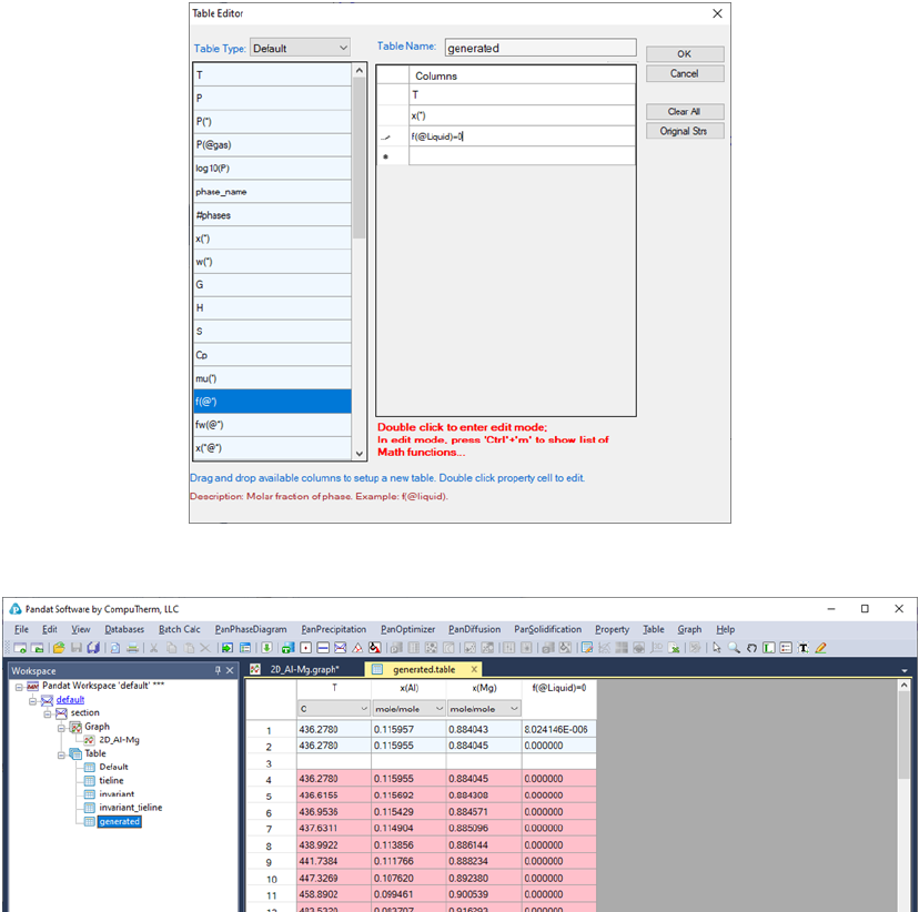
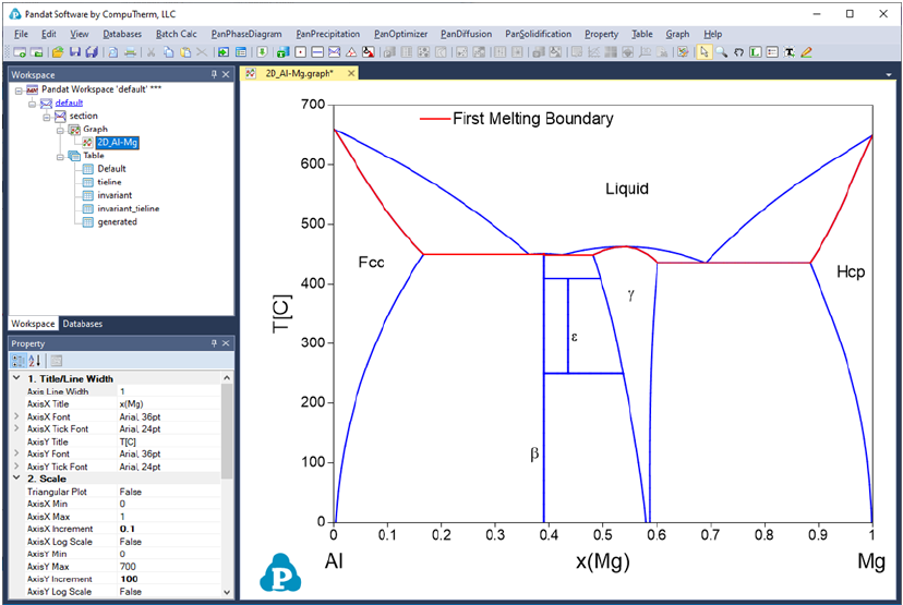
Here an example is given to demonstrate how to use the logical expression to
obtain useful information from the calculated results. Figure 2.26 shows the
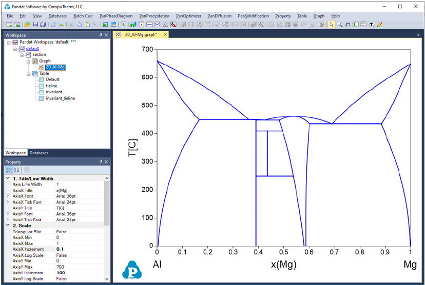
36
calculated Al-Mg binary phase diagram. After the calculation, a table is
generated with the constraint of f(@Liquid)=0, as seen in Figure 2.27. The
new generated table is shown in Figure 2.28, which is a subset of the phase
boundaries of Al-Mg where liquid phase exists and has phase fraction of zero,
the so-call “first melting” boundary. This set of boundaries can be plotted on
the Al-Mg phase diagram following the approach in Section 2.3.3. The first
melting line is shown in red as in Figure 2.29. More examples will be presented
in Section 3.3.8.
Figure 2.26 Calculated Al-Mg binary phase diagram
37
Figure 2.27 Generating a new table with a constraint of f(@Liquid)=0
Figure 2.28 The generated table with the constraint of f(@Liquid)=0
38
Figure 2.29 The first melting boundary merged on the Al-Mg phase diagram
2.5 Console Mode
In addition to the most common GUI (graphical user interface) mode, Pandat
TM
can also run in the console mode without opening GUI. There are two ways to
activate the console mode:
(1) double click a batch file (extension with pbfx) in a folder, or
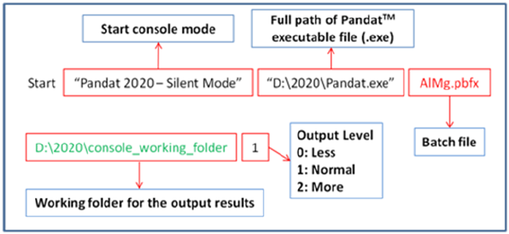
(2) run through a windows bat file. The content of an example bat file is
shown below:
39
Figure 2.30 Example of the (.bat) file for console mode
The command is to start Pandat
TM
(with full path and titled as “Pandat 2020 -
Silent Mode”) and run the batch file AlMg.pbfx (in the current folder if not in
full path). The last two arguments are optional. If a working folder is given
(“D:\2020\console_working_folder”), a Pandat
TM
workspace is created in the
folder and all simulation results are saved under the workspace. The
simulation progress is logged in the file “pandat.log”. The last argument is to
control the output level with “1” the default value. The value of “2” is for more
outputs and “0” for less. Please refer to example #29 in Example Book for more
detail information.