239
9 High-Throughput-Calculation
The High-Throughput-Calculation (HTC) function has been implemented in
Pandat
TM
for the PanPhaseDiagram, PanPrecipitation, and PanSolidification
modules. It can perform thousands of calculations in a user defined
compositional space by a simple setting. Alloy compositions that satisfy user
defined criteria can then be identified through mining the thousands of
simulated results. This function allows user to develop alloys with certain
properties through design. There are two methods to define alloy compositions
for HTC: one is to setup the composition range of each component and its steps
through user-interface; the other one is to load the user-defined composition
data file. These two methods will be explained in detail in this section. Note
that, the current HTC function can carry out 0D-point calculation and
solidification simulation using both the Scheil and Lever-rule models in the
PanPhaseDiagram module. In the PanPrecipitation module, HTC can be carried
out for all defined/imported alloys under one or multiple heat-treatment
conditions. The HTC function is also available in the newly developed
PanSolidification module for alloys under different cooling rates. The tutorial of
the HTC function in different modules will be given in this section as well.
Other types of simulations will be continuously developed in the future.
9.1 Alloy Composition Setup
9.1.1 Setting Composition Range and Steps
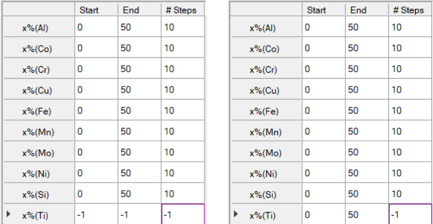
The composition setup dialog for the HTC function in different modules is the
same. As shown in Figure 9.1, the composition range of each component can
be defined by using the Start and End values. The #steps define the
composition increment from the Start value. Note that the End value will
always be selected even it may not be the same as the last value calculated by
the defined composition increment. In this example, the composition of Ti is set
240
as the balance by right-click the row of Ti (a) or typing in the Ti composition
rang and “-1” for steps (b).
Figure 9.1 HTC composition setup dialog
9.1.2 Import Alloy Compositions
Pandat also allows user to import alloy compositions for HTC through a data
file. This is a more flexible and efficient way to perform HTC for a group of
multi-component alloys which may contain different alloying elements. The
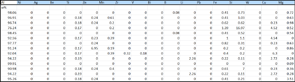
format of a data file (.txt or .dat) is simple. Figure 9.2 shows an example which
contains a group of Al-rich alloys. The first row shows all alloying elements
involved in these alloys. The first column of the second row defines the unit of
the alloy composition. Then alloy compositions are given from the third row
forward. There are a few points to emphasize here:
1. The element in the first column is automatically treated as “balance”
element, such as Al in this example. No matter what values are given in
the first column, those values will be recalculated after the compositions
of all other components are read in.
2. The first row lists all the elements used in the alloys. The compositions of
some of them can be zero in a certain alloy.
(a)
(b)
241
3. If an alloying element is not available in the database used to perform
HTC, this element will be kicked out in the calculation and its
composition will be automatically added to that of the “balance” element.
Figure 9.2 Example of composition file for multi-component Al-rich alloys
242
9.2 HTC Tutorial in PanPhaseDiagram
In this example, we will demonstrate how to calculate liquidus, solidus, and
solidification ranges for a number of Al-Mg-Zn alloys via the HTC function by
setting composition range and steps.
1. Load proper database and choose the Al-Mg-Zn system.
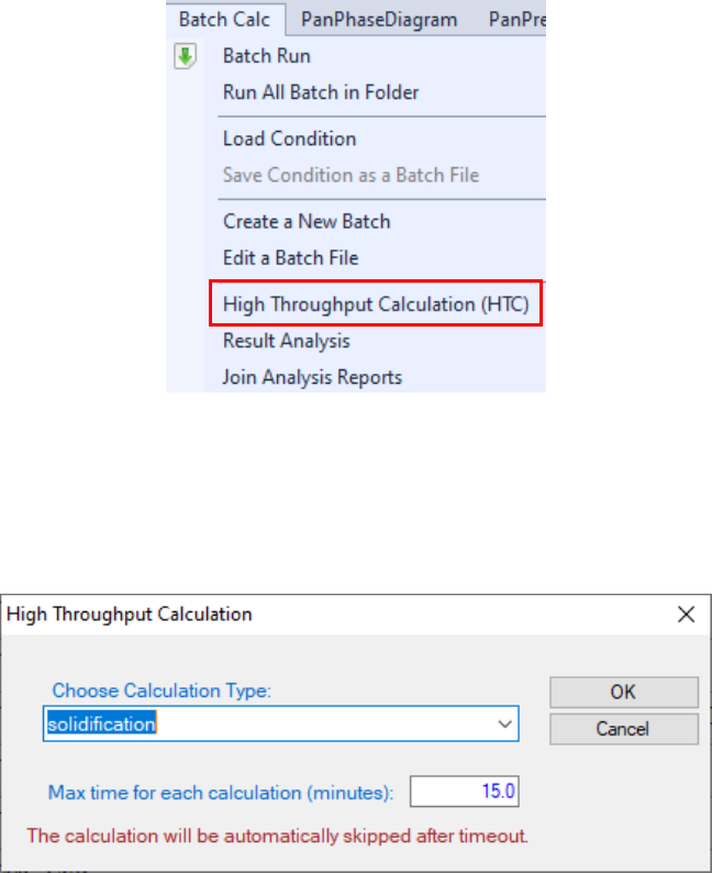
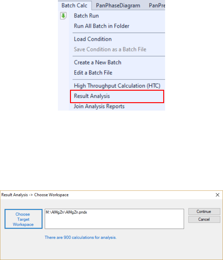
2. Choose the HTC function from the Batch Calc → High Throughput
Calculation (HTC) (as shown in Figure 9.3).
Figure 9.3 HTC function under the “Batch Calc” menu
3. Choose the calculation type from the drop-down list of HTC pop-up
window and select “Solidification”.
Figure 9.4 Dialog to choose calculation type of HTC
4. Define the compositional space for HTC simulation.
243
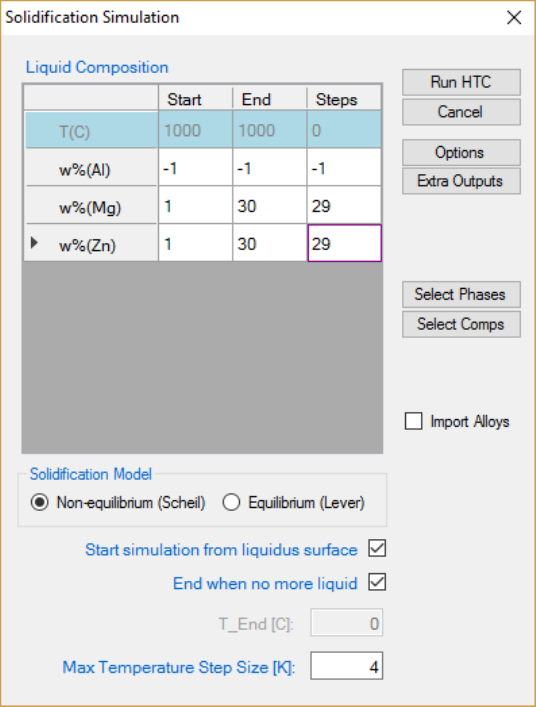
After step 3, a window pops out as shown in Figure 9.5. In this setting, the
compositions of both Mg and Zn vary from 1 to 30 wt.% in a double
composition loops. The “Steps” is set to 29, which means the composition
increases by 1 wt% at each step. The total number of calculations is
3030=900 in this setting. The composition of Al is set as balance by typing “-1”
for steps or right-click the row of Al. No “Start” or “End” values are required for
the balance component, which is Al in this case. After setup the compositional
space for HTC and choose the proper solidification model, user can click “Run
HTC” button to perform HTC simulations, which is 900 calculations in this
case.
Figure 9.5 Dialog to setup compositional space for HTC
5. Save the current workspace after all calculations are finished. It is
suggested that user saves the current workspace immediately after the
244
HTC calculation. This allows all the calculated results saved in the
workspace for future use.
6. Choose “Result Analysis” from the “Batch Calc” menu. User can use
this commend to analyze the calculated results for a group of alloys and
choose a certain property from each calculation for comparison.
Figure 9.6 “Result Analysis” function under the “Batch Calc” menu
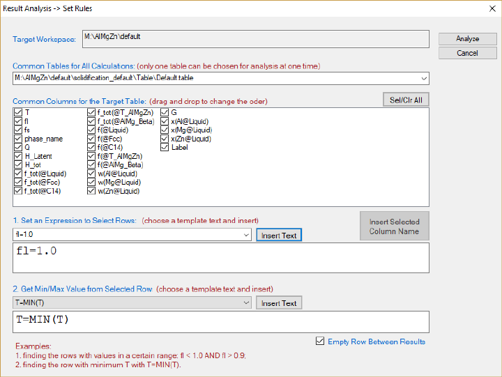
7. Open the workspace saved previously for “Result Analysis”. User can
perform several HTC calculations and save all the workspaces. User can
then analyze the results of the selected HTC calculation by opening the
corresponding workspace as shown in Figure 9.7.
Figure 9.7 “Result Analysis” popup dialog to choose target workspace
8. Define the criteria of the properties as filters for result analysis.
245
Figure 9.8 “Result Analysis” popup dialog to define the criteria of the properties
In Figure 9.8, the “Target Workspace” shows the workspace selected by the
user for results analysis. It should point out that there can be more than one
table in each calculation, the “Common Tables for All Calculations” allows user
to choose the table for analysis. In the “Common Columns for the Target Table”
window, names for all the output properties available in the selected table are
listed. User can choose the properties to be listed in the “Analysis Report”. As
shown in Figure 9.9, temperature and the alloy composition will be listed in the
“Analysis Report” in this case. Since the purpose of HTC is to compare a special
target property for the several hundred/thousands of calculations, the “Set an
Expression to Select Rows” at the bottom of the window allows user define the
criteria. In Figure 9.9, this criterion is f
L
=1, i.e. the fraction of liquid is 1. With
this filter, only the row satisfies this criterion will be listed in the “Analysis
Report”. It should point out that several criteria can be set in the “Set an
Expression to Select Rows”. Click “Analyze” to create the “Analysis Report” as
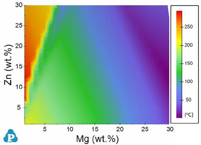
shown in Figure 9.9. In this table, each row lists the liquidus temperature for
the corresponding alloy composition. The liquidus temperatures for 900 alloys
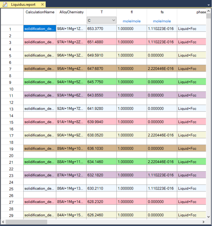
247
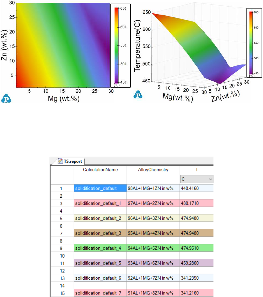
Figure 9.10 3D diagrams of the liquidus temperatures: colormap (left) and 3D
surface (right)
9. Save the obtained T
L
report file via “File → Save Current File As”.
10. Now repeat the steps of 1-8 to obtain the T
S
report file and save it.
Figure 9.11 Analysis report file of solidus temperature T
S
11. Combine the two analysis reports. Note that user can also easily export
the obtained report file to excel (Table → Export to Excel) for further
editing and then import the modified file back to Pandat
TM
to create plot.
For example, we can export the T
L
and T
S
reports to excel files and then
249
9.3 HTC Tutorial in PanPrecipitation
In this example, we will demonstrate how to find the peak yield strength of the
AA6005 alloy with varying both composition and heat-treatment temperature.
1. Load proper thermodynamic + mobility database and select Al, Mg, Si
three components.
2. Load proper kinetic-parameter database to select the matrix phase and
precipitates.
3. Choose the HTC function from the Batch Calc → High Throughput
Calculation (HTC).
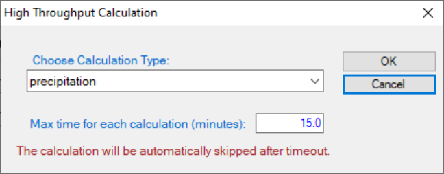
4. Choose the calculation type from the drop-down list of HTC pop-up
window and select “Precipitation”.
Figure 9.13 Dialog to choose calculation type of HTC
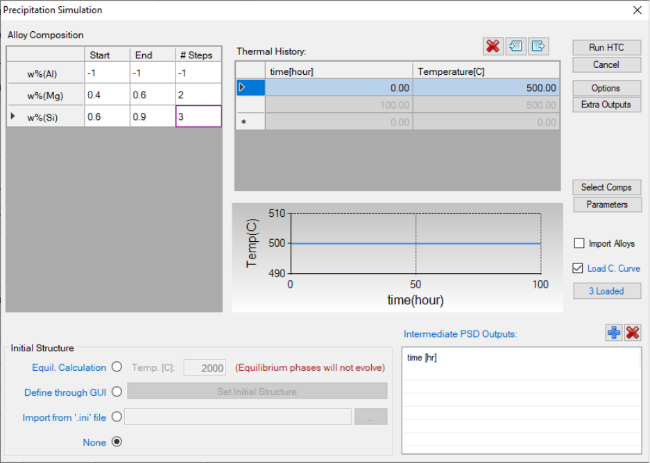
5. Define the compositional space for HTC simulation. As shown in Figure
9.14, the compositions of Mg and Si varying within the ranges of 0.4-0.6,
and 0.6-0.9 (wt.%), respectively.
6. Define the thermal history for HTC simulation. User can define/import
one thermal history by using the “Thermal History” dialog in Figure
9.14 or select the “Load C. Curve” and click the “Import CC” button to
browse and load the predefined cooling curves (.txt or .dat). The example
format of cooling curve file can be found in Figure 9.21 in section 9.x.x.
In this example cooling curves, isothermal aging for 20 hours at three
temperatures 190, 182, and 170
o
C are defined individually.
250
7. In addition to use the default output, user can also customize the
outputs using the “Extra Outputs” function. In this example, the extra
output with time, T - temperature, w(*) - alloy composition, and sigma_y
(yield strength) is generated.
8. After setup the compositional space for HTC and define/import the
proper thermal history , user can click “Run HTC” button to perform
HTC simulations.
Figure 9.14 Dialog to setup compositional space and thermal history for
precipitation HTC
9. Save the current workspace after all calculations are finished and run
“Result Analysis” from the “Batch Calc” menu. User can use this
commend to analyze the calculated results for a group of alloys and pick
a certain property from each calculation for comparison. As shown in the
following Figure 9.15, the following rule is used to obtain the maximum
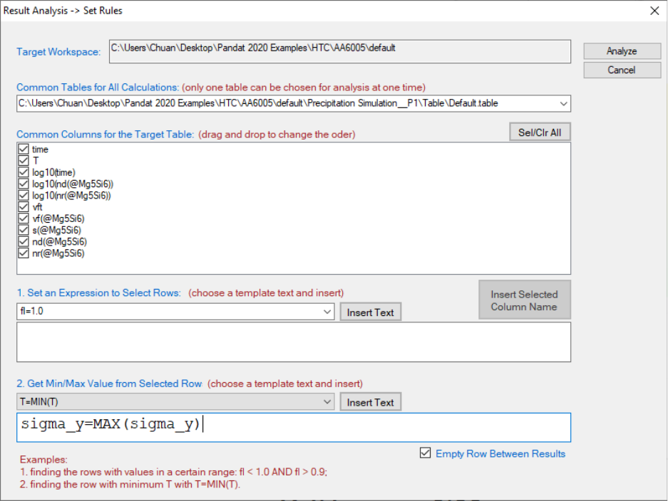
251
yield strength of each alloy under thee different heat treatment
conditions.
Figure 9.15 Criteria for precipitation results analysis
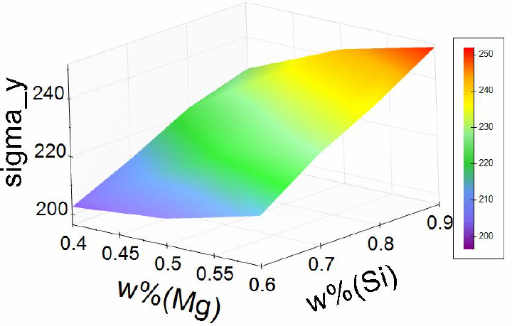
Figure 9.16 shows the obtained peak yield strength distribution within the
defined composition space considering all three heat treatment conditions.
User can run “Result Analysis” on this save workspace and dig out more
information using other rules. For example, user can plot peak yield strength
distribution in the composition space for one particular heat treatment
condition.
252
Figure 9.16 The maximum yield strength distribution within the defined
compositional space
253
9.4 HTC Tutorial in PanSolidification
Hot tearing or hot cracking is a serious defect occurred in welding and casting
solidification. Cracking usually generated at the end stage of solidification
along grain boundaries. Prof. Kou [2005Kou] proposed a criterion to describe
the crack susceptibility by using a simple crack susceptibility index (CSI),
which is the maximum value of |dT/d(f
s
)
1/2
| at f
s
1/2
< 0.99. The CSI criterion
has been successfully applied to several Al-based alloy systems. In this
example, we will demonstrate how to use HTC function in PanSolidification
module to produce a susceptibility map in the Al-Cu-Mg ternary system.
1. Create a workspace and select PanSolidification module. Save the
workspace in a user assigned folder different from that of the default
workspace. The HTC calculation results will be saved automatically
under this folder.
2. Load proper thermodynamic + mobility database and select Al, Cu, Mg
three components.
3. Load proper solidification kinetic-parameter database (.sdb) to select the
solidification alloy system.
4. Choose the HTC function from the Batch Calc → High Throughput
Calculation (HTC).
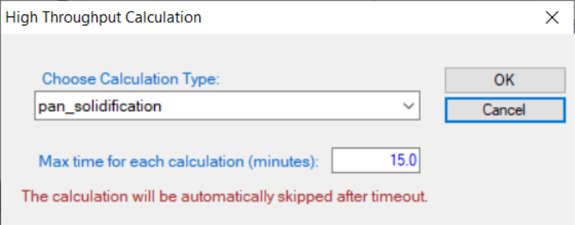
5. Choose the calculation type from the drop-down list of HTC pop-up
window and select “pan_solidification”.
254
Figure 9.17 Dialog to choose calculation type of HTC in PanSolidification
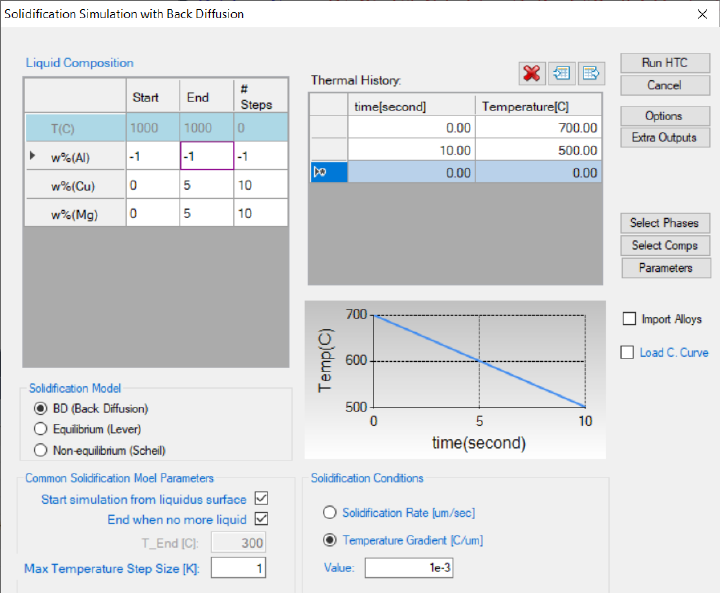
6. Define the compositional space for HTC simulation. As shown in Figure
9.18, the compositions of Cu and Mg varying within the ranges of 0-5,
and 0-5 (wt.%), respectively.
7. Define the solidification conditions for HTC simulation. User can
define/import cooling rate (the example is 20 K/s) by using the “Thermal
History” dialog in Figure 9.18 or select the “Load C. Curve” and click
the “Import CC” button to browse and load the predefined cooling curves
(.txt or .dat). The example format of cooling curve file can be found in
Figure 9.21. Besides the cooling rate, the solidification rate or
temperature gradient is also needed to be defined.
Figure 9.18 Dialog to setup compositional space and solidification conditions
for PanSolidification HTC.
8. In addition to use the default output, user can also customize the
outputs using the “Extra Outputs” function. In this example, we defined
the following extra output: time; T – temperature; w(*) – alloy composition;
255
fs – solid phase fraction; sqrt(fs) – the square root value of the solid
phase fraction; and -T//sqrt(fs) – the CSI index |dT/d(f
s
)
1/2
| because
T//sqrt(fs) is a negative value.
9. After setup the compositional space for HTC and define/import the
proper thermal history (as shown in Figure 9.18), user can click “Run
HTC” button to perform HTC simulations.
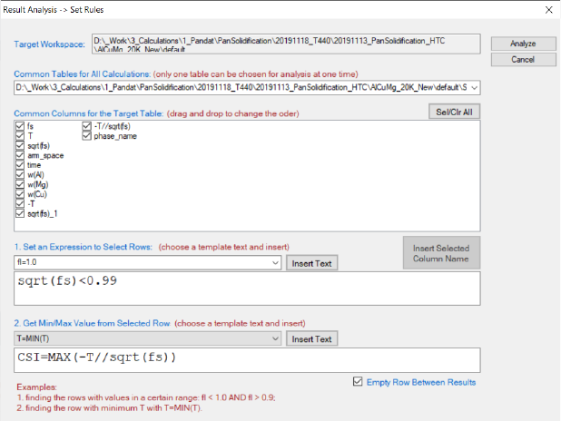
10. Run “Result Analysis” from the “Batch Calc” menu. User can use this
commend to analyze the calculated results for a group of alloys and pick
a certain property from each calculation for comparison. As shown in the
following Figure 9.19, the criterion is to output the MAX(-T//sqrt(fs)) at
each composition point.
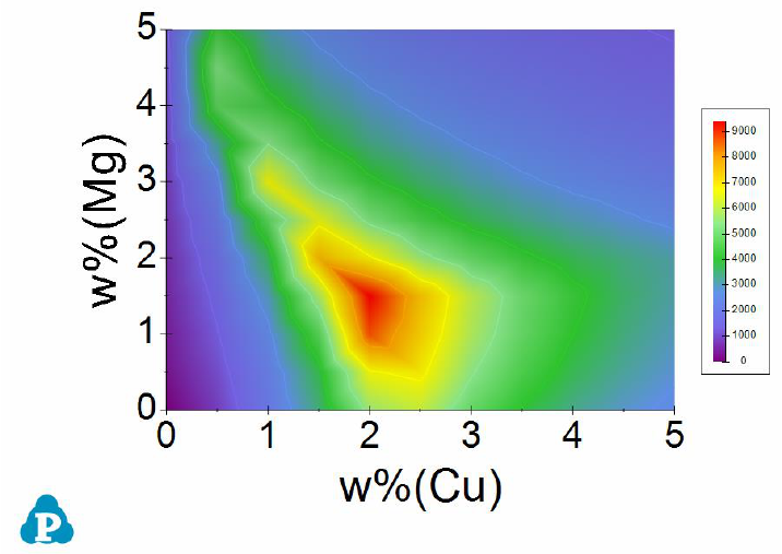
11. Figure 9.20 shows the obtained crack susceptibility map for Al-Cu-Mg
alloys with cooling rate of 20 K/s. User can run “Result Analysis” on
this save workspace and dig out more information using other rules.
Figure 9.19 Criteria for Cracking Susceptibility Index setting from solidification
results analysis.
256
Figure 9.20 Al-Cu-Mg crack susceptibility map with cooling rate of 20 K/s.
257
9.5 Run HTC in Console Mode
In order to facilitate the integration of PanPrecipitation with a third-party
software package such as iSight or DEFORM, a new feature is developed so that
the software can call PanPrecipitation for multiple simulations with different
conditions. In this case, PanPrecipitation run in a console mode rather than in
a regular GUI mode. This would significantly reduce the overhead from creating
and maintaining many GUI components. In this mode, the simulation is
performed through a script file or Pandat batch file (.pbfx file). After the
simulation is done, the results are saved as ASCII files, which can then be
loaded by third-party software package for subsequent simulations.
A typical application of this function is to run HTC of an alloy at various
cooling profiles. The command to run this type of precipitation HTC is:
Pandat.exe Ni-14Al.pbfx “D:\ConsoleMode\results” cooling_curve.txt 1
There are four arguments passed to Pandat.exe in order to run HTC:
a) Ni-14Al.pbfx: batch file name, which defines all the simulation
conditions such as unit, alloy chemistry, output format, etc.; The heat
treatment schedule will be replaced by the 3rd argument if there is
cooling curve file attached;
b) "D:\ConsoleMode\results": working folder for Pandat HTC. A default
workspace will be created automatically when running Pandat each time.
The old workspace will be removed in this folder. If the user wants to
keep the workspace and its results, all the files in this folder should be
backed up before running HTC each time. Or the user may specify a
different working folder for each HTC calculation;
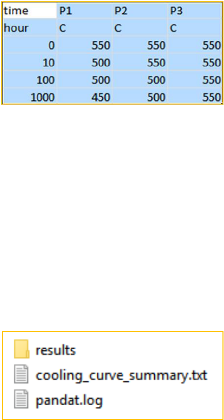
c) cooling_curve.txt: the files defining cooling curves for different points.
The file format is Tab Delimited text file.
258
Figure 9.21 The example file format defining cooling curves for different points
The following is the structure of the working folder (see Figure 9.22):
1. Workspace folder: contains all the results for each simulation;
2. “cooling_curve_summary.txt”: the summary file which contains the results
for the final step of each simulation; if there are multiple tables in pbfx file,
only the results from the last table is summarized; the file format is Tab
Delimited text file;
3. pandat.log: which logs the simulation progress; the level can be controlled
by the last argument as shown above.
Figure 9.22 The structure of the working folder.
Please refer to Pandat Examples\ConsoleMode for more detail information.