173
6 PanDiffusion
PanDiffusion is a module of Pandat
TM
software designed to simulate kinetic
processes dominated by elemental diffusion. PanDiffusion provides a rich
variety of applications including particle dissolution, carburization,
decarburization, homogenization, phase transformation, diffusion couple, and
so on.
PanDiffusion is seamlessly integrated with the user-friendly Pandat
TM
Graphical User Interface (PanGUI) as well as thermodynamic calculation engine,
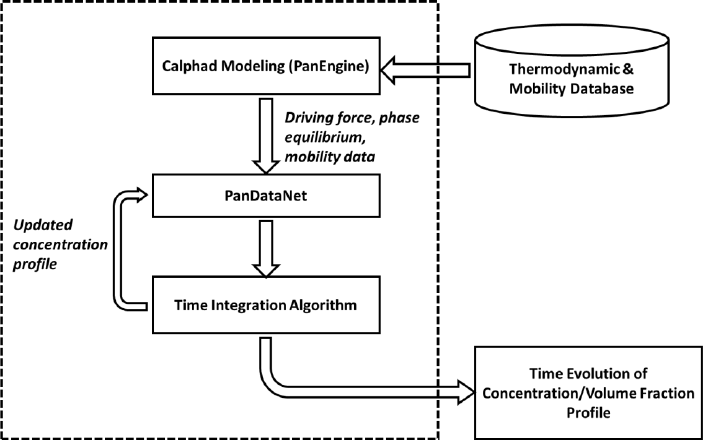
PanEngine. The interface between PanDiffusion and PanEngine is managed
through PanDataNet. The implementation of PanEngine guarantees reliable
input data, such as chemical potential, phase equilibrium and mobility. Figure
6.1 shows an overall architecture of the PanDiffusion module.
Figure 6.1 An overall architecture of the PanDiffusion module
174
6.1 Features of PanDiffusion
6.1.1 Overall Design
➢ Time evolution of composition profile, phase volume fraction, and phase
composition.
➢ Multiple selections of thermal history, boundary condition and geometry.
➢ Applications including particle dissolution, carburization,
decarburization, homogenization, phase transformation, and diffusion
couple.
6.1.2 Kinetic Model
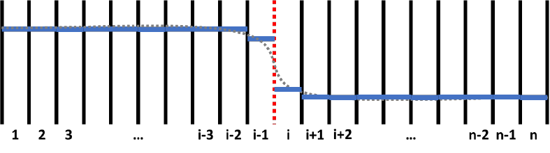
Figure 6.2 shows a schematic plot of a composition profile in a diffusion couple.
In the simulation, the sample is divided by grids with equal width. The
numbers, 1, 2, 3, …, n, indicate grid id. The solid black and dashed red lines
means inter-grid interface. What is more, the red dashed line between (i-1)-th
and i-th grids indicates the position of a sharp interface of this diffusion couple.
Inter-grid flux is calculated following Fick’s first law. Composition of each grid,
which is indicated by solid blue line in Figure 6.2, is calculated following Fick’s
second law. The discrete composition profile represents a continuous
composition profile of grey dashed line. Chemical potential, mobility, phase
equilibrium and related properties are updated for each grid after calculating
the composition.
Figure 6.2 A schematic plot of a composition profile in a diffusion couple

175
6.1.2.1 Flux Model
The evolution of each grid’s composition is controlled by the inter-grid flux
which is calculated based on absolute reaction rate theory [1941Gla]. At the
lattice-fixed frame of reference, the flux is:
(6.1)
Where
is the flux of -th element between the grid and the grid .
is
effective mobility, is the gas constant, T is temperature in Kelvin,
is molar
volume, is the thickness of grid interface and in most cases calculated as
average grid size,
and
are molar fraction of k-th element at the grid
and the grid ,
is the chemical potential difference of k-th element
between the grid and the grid . The sinh is the hyperbolic sine function.
For convenience of calculation, a composition profile is observed at a volume-
fixed frame of reference, and the flux of substitute element is transformed to
.
Then the amount of k-th element (
) of each grid can be updated according
Fick’s 2
nd
law:
(6.2)
Where unit normal vectors point outward from the grid.
176
6.2 Get Started
6.2.1 Step 1: Create a PanDiffusion Project
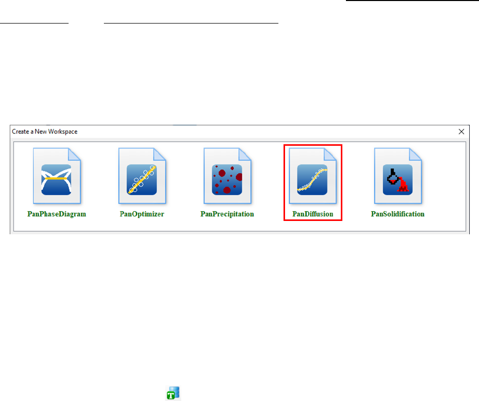
Users can create a PanDiffusion project through menu “File → Create a New
Workspace” or “File → Add a New Project” in an existing workspace. The
“Module Window” pops out for user to choose a module for the new project as
shown in Figure 6.3. Choose “PanDiffusion” module for diffusion simulation,
and the PanDiffusion project will be created after user click on Create button
or double click on the PanDiffusion icon.
Figure 6.3 Creating a PanDiffusion workspace
6.2.2 Step 2: Load Thermodynamic and Mobility Database
The next step is to load the database, which is FeCrNi.tdb in this example.
Different from the normal thermodynamic database, this database also
contains mobility data for the phases of interest in addition to the
thermodynamic model parameters. Both are needed for carrying out diffusion
simulation. By clicking the button on the toolbar, a popup window will open,
allowing user to select the database file.
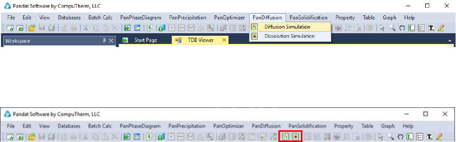
6.2.3 Step 3: Start PanDiffusion Module
Perform diffusion simulation through manual bar PanDiffusion->Diffusion
Simulation or tool bar as shown in Figure 6.4 and Figure 6.5.
178
6.3 Tutorial 1: Diffusion Couple with
Uniform Composition Input
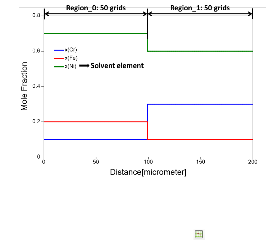
In this tutorial, the diffusion simulation on a diffusion couple with uniform
composition at each side (as shown in Figure 6.6) is carried out. The annealing
temperature is 1000
o
C and the duration is 2 hours. “Region_1” represents the
left-hand side of this diffusion couple, and “Region_2” represents the right-
hand side of this diffusion couple. Each region is 100μm and the simulation
box is discretized to 100 grids.
Figure 6.6 Initial conditions of the diffusion couple simulation.
6.3.1 Set up initial condition for diffusion simulation
In order to set the above conditions in PanDiffusion, click through the menu
“PanDiffusion → Diffusion Simulation” or click the button on the tool bar,
a popup window will show and allow users to set up calculation conditions (as
shown in Figure 6.7 and Error! Reference source not found.).
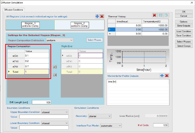
179
Click Region_1 to set up the composition of the left-hand side as shown in
Figure 6.7, and click Region_2 to set up composition of the right-hand side as
shown in Error! Reference source not found.. Details regarding the interface
design will be described in Section 6.5. Constant annealing temperature is set
as 1000
o
C, and annealing time is 2 hours.
Figure 6.7 Dialog window for user to set the composition of Region_1
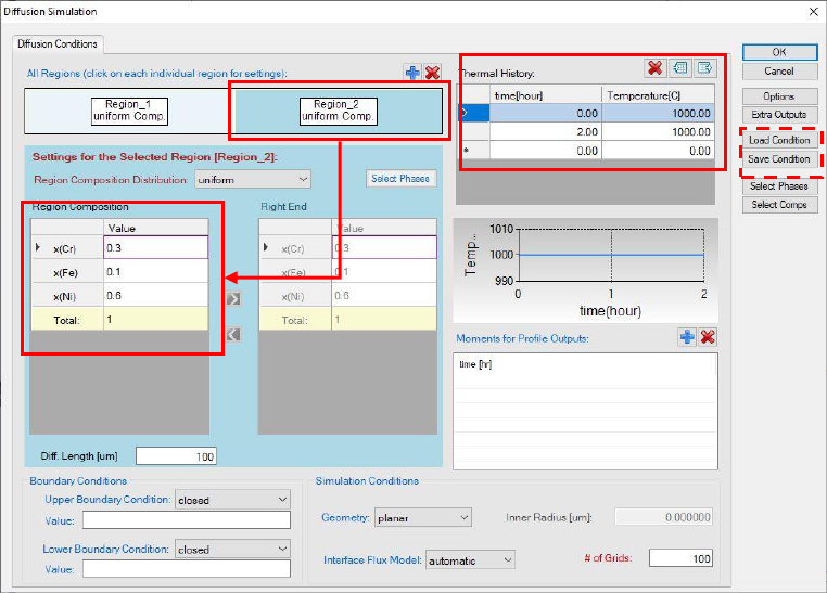
180
Figure 6.8 Dialog window for user to set the composition of Region_2 and
diffusion simulation conditions
As is highlighted by the dashed box, the simulation condition can be saved to a
“.pbfx” file by selecting “Save Condition”. The saved condition can be loaded by
clicking “Load Condition” for the future usage. When a condition is loaded from
“.pbfx” file, the settings in the GUI are updated accordingly.
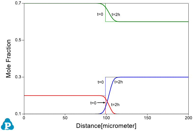
6.3.2 Simulation results
Click OK button in Error! Reference source not found. to start the
simulation after the initial condition is set properly. The simulation result is
displayed in Figure 6.9.
Click it
181
Figure 6.9 Output graph showing the initial and final composition profiles.
In this case, only the initial and final composition profiles are presented: the
dotted lines with sharp interface are for the initial stage and the solid lines with
smooth interface are for the final stage.
6.3.3 Customize Simulation Results
As all other calculations available in Pandat
TM
, upon the completion of the
diffusion simulation, a default table of properties (such as time, temperature,
grid size, distance, composition distribution, volume fraction and chemical
potential) is automatically generated and a default graph of composition
profiles is displayed. User can refer to sections 2.3 and 2.4 to learn how to
customize simulated graph and table.
182
6.4 Tutorial 2: Diffusion Simulation
with Composition Profile Input
In this tutorial, the Fe-Ni-Cr alloy is taken as an example to demonstrate a
diffusion simulation with a composition profile input. The format of input file is
discussed in section 6.6.3. The database file mentioned in this section,
“FeCrNi.tdb”, can be found in the installation folder of Pandat
TM
. In general,
user should follow the following steps to carry out a diffusion simulation:
6.4.1 Set up initial condition for diffusion simulation
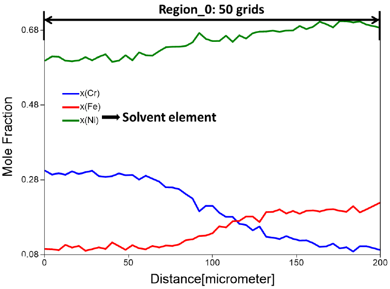
Figure 6.10Error! Reference source not found. demonstrates the conditions
of this simulation. The initial composition profile from the input file is
displayed in this figure. The length of the profile is 200um and is discretized to
100 grids.
Figure 6.10 Initial conditions of the diffusion simulation with a composition
profile input.
183
To set the above conditions in PanDiffusion, click through on the tool bar,
or from the menu “PanDiffusion → Diffusion Simulation” a popup window as
shown in Figure 6.8Error! Reference source not found. will allow users to set
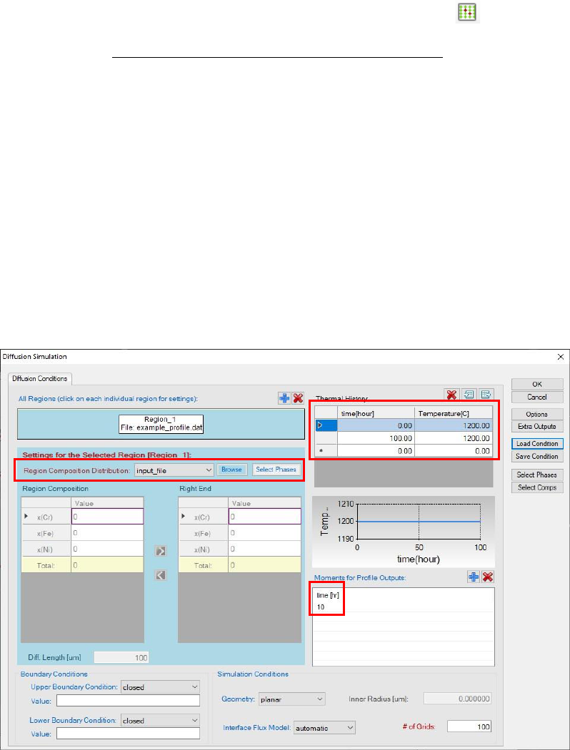
up calculation conditions. In Figure 6.11Error! Reference source not found.,
“Region_2” is deleted firstly. Please refer to section 6.6.4 on how to delete a
region. In the remaining “Region_1”, select “input_file” from “Region
Composition Distribution”, and click “Browse” to load a .dat (or .txt) file which
contains composition profile. Annealing time (100 hours in total) and annealing
temperature (1200
o
C) are set. Add an intermediate output at 10 h in the
“Moments of Profile Outputs” to observe simulation process. Please refer to
section 6.6.8 on how to add a moment of profile output.
Figure 6.11 Dialog window for user to input diffusion simulation conditions
and composition of Region_1.
6.4.2 Simulation results
Click OK button in Error! Reference source not found. to start the
simulation after the initial condition is set properly. The simulation result is
184
displayed in Figure 6.12. Please refer to section 2.3 of this user manual to add
text, legend, and change the appearance of the figure.
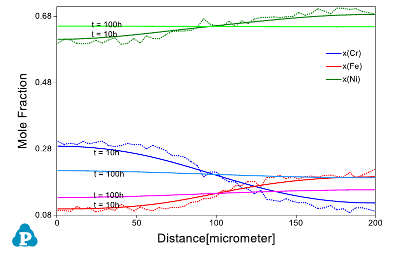
Figure 6.12 Output graph showing the initial and final composition profiles
As is seen in this figure, the initial serrated composition profiles were smoothed
out after 10 hours of annealing at 1200
o
C, and the material is homogenized
after 100 hours of annealing.

185
6.5 Tutorial 3: Dissolution Simulation
In this tutorial, the Al-Cu alloy is taken as an example to demonstrate a
dissolution simulation. The GUI of dissolution is discussed in section 6.7. In
general, user should follow the following steps to carry out a dissolution
simulation:
6.5.1 Set up initial condition for dissolution simulation
The particle is assumed to be spherical and have a radius of 3 um, and its
volume fraction is 0.008. The overall composition of the system is 98.45Al-
1.55Cu (at%). The simulation box is digitized to 100 grids.
To set the above conditions in PanDiffusion, click on the tool bar, or from
the menu “PanDiffusion → Dissolution Simulation” a popup window as
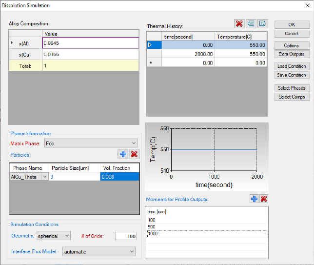
shown in Figure 6.13 will allow users to set up calculation conditions. In “Alloy
Composition” section, the overall composition of Al-Cu alloy is set to 98.45Al-
1.55Cu (at%). In “Phase Information” section, set “Matrix Phase” as Fcc. In
“Particles” subsection, click bottom to add a particle, set “Phase Name” as
AlCu_Theta, set “Particle Size” as 3 um, and set “Vol. Fraction” as 0.008. In
“Simulation Conditions” Section, set “Geometry” as spherical, and set “# of
Grids” as 100. In “Thermal History” section, temperature is set as 550
o
C, and
heat treatment duration is set as 2000 seconds.
Add additional intermediate outputs at 100s, 500s and 1000s in the section
“Moments for Profile Outputs”, then click “OK” to start the calculation
186
Figure 6.13 Dialog window for user to input dissolution simulation conditions.
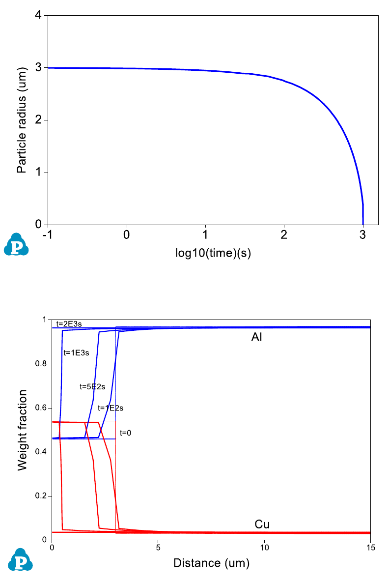
6.5.2 Simulation results
Click OK button in Figure 6.14 to start the simulation after the initial condition
is set properly. The simulation results are displayed in Figure 6.15 and Figure
6.15. Please refer to Section 2.3 of this user manual to add text, legend, and
change the appearance of the figure. Figure 6.14 shows the particle size change
with time, from 3m (radius) at beginning to zero after annealing at 550
o
C for
~1000 seconds. Figure 6.15 shows diffusion between particle and matrix and
the composition profiles at 0s, 100s, 500s, 1000s, and 2000s. It is seen from
Figure 6.15 that the particles are completely dissolved after annealing for
2000s.
187
Figure 6.14 Output graph showing the time evolution of particle radius
Figure 6.15 Output graph showing the time evolution of composition profile.
188
6.6 Settings in General Simulation GUI
User can perform variety of diffusion simulations by PanDiffusion module. All
types of simulations, except for particle dissolution, share the same general
graphic user interface (GUI) to set up simulation conditions. This GUI can be
accessed through manual bar PanDiffusion->Diffusion Simulation, or by
clicking on the Toolbar. The speial GUI for dissolution simulation can be
accessed through PanDiffusion->Dissolution Simulation, or by clicking on
the Toolbar. We will present the features of the general GUI in this section.
6.6.1 Set Units
In the GUI of PanDiffusion, unit settings can be accessed through “Options-
>Calculation->Units”. Please refer to section 3.2.2 for details.
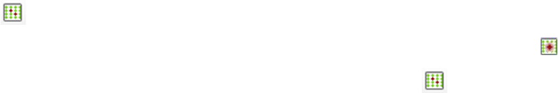
6.6.2 Select Phases
By clicking “Select Phases” as highlighted by the red box in Figure 6.16, user
can select phases involved in the diffusion simulation on the system level. By
default, all the phases in the alloy system are selected, while user can deselect
some of them as wishes. In addition, user can also select phases for each
region by clicking “Select Phases” as highlighted by the green box in Figure
6.16. By default, phase selection for each region follows the global setting in
the system level.
189
Figure 6.16 Select phases in a system and/or in a region
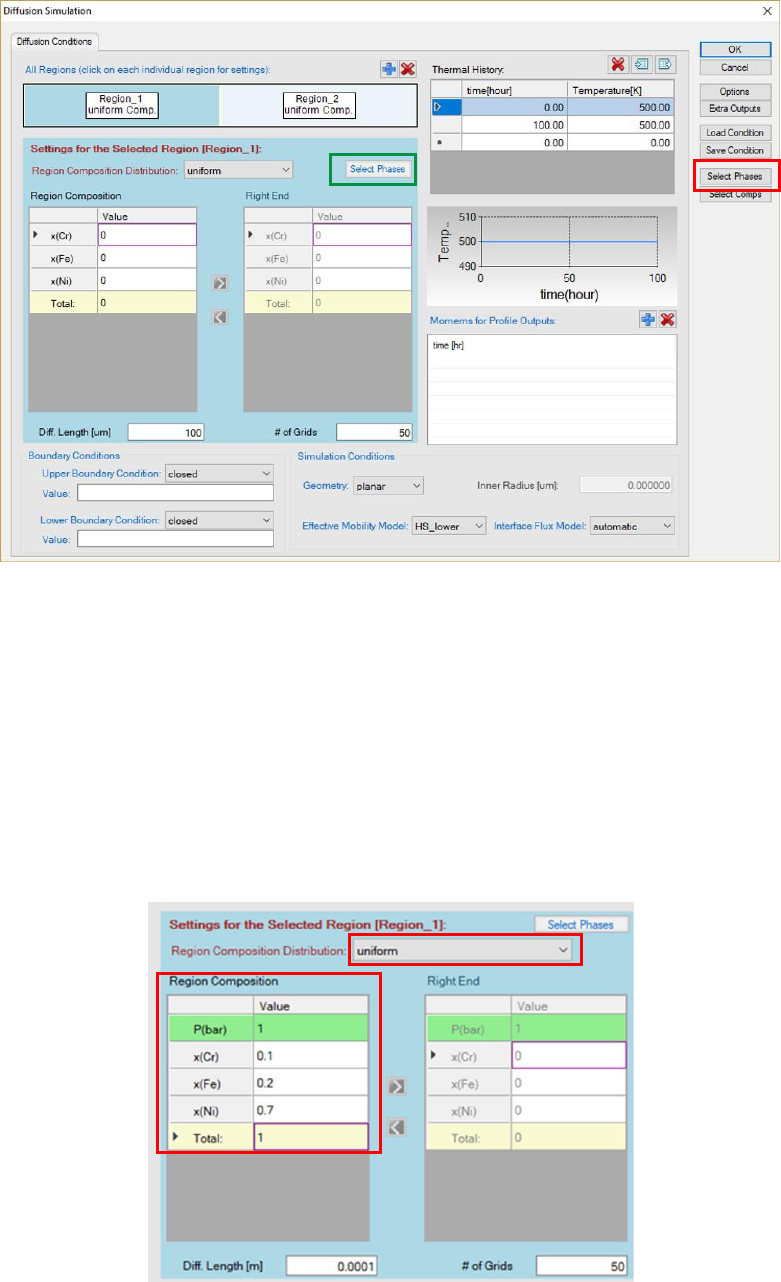
6.6.3 Set Initial Composition Profile
In the GUI of PanDiffusion, initial composition profile is assigned region-by-
region. In each region, composition profile can be:
• Uniform: the composition of each element in the selected Region is a
constant. When “uniform” is selected, a homogenous “Region
Composition” can be set.
190
Figure 6.17 “Uniform” composition of a Region
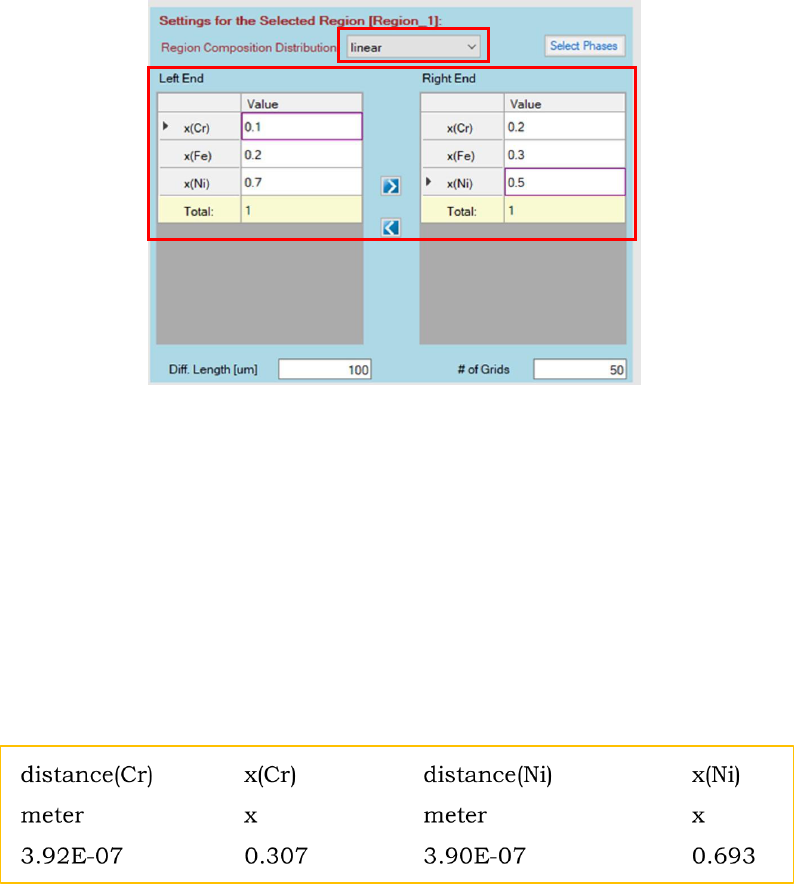
• Linear: a linear composition interpolation is set from the left edge to the
right edge of the selected Region. When “linear” is selected, both “Left
End” and “Right End” compositions need to be set.
Figure 6.18 “Linear” composition of a region
• Input_file: Load composition profile from a tab-delimited .dat (or.txt) file
with the following two kinds of formats:
Format (I): the distance is specified for each element, which is usually
the case when using experimental data. The 1
st
row contains the name of
each column, the 2
nd
row contains the unit definition, and value starts
from the 3
rd
row.
Format (II): the distance is specified in the 1
st
column, the composition of
every element correspond to the same distance. This format is usually
obtained by digitalizing data from literature. The 1
st
row contains the
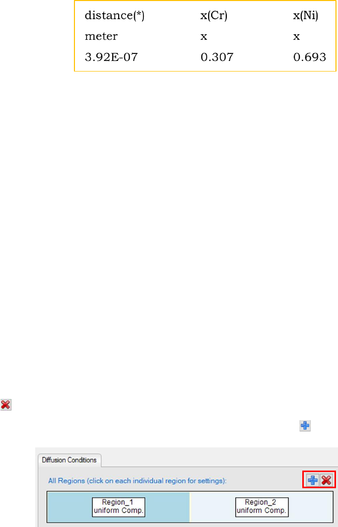
191
name of each column, the 2
nd
row contains the unit definition, and value
starts from the 3
rd
row.
The unit of distance can be: meter (or m), millimeter (or mm), micrometer (or
um), nanometer (or nm) and angstrom. The unit of composition can be: x for
mole fraction, x% for mole percentage, w for weight fraction, and w% for weight
percentage. Note that, the units in the input file will override setting in
“Options->Calculation->Units” and the input file is case insensitive.
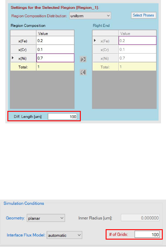
6.6.4 Delete and Add a Region
In the GUI of PanDiffusion, there are two Regions by default. In the following
cases, single region is recommended:
• Only one input composition profile
• Carburization, decarburization, or other surface flux process, with a
homogeneous initial composition profile
• Homogenization of a linear composition profile
The redundant region can be removed by first selecting the Region, then
clicking button as shown in Figure 6.. If diffusion is among three or more
Regions, Regions can also be added one by one by clicking .
Figure 6.19 Add or delete a region
192
6.6.5 Set Regional Length
In the GUI of PanDiffusion, “Diff. Length” is the length of a region.
Figure 6.19 Length in a region
6.6.6 Set # of Grids
In the GUI of PanDiffusion, number of grids is set for the entire simulation box
and is distributed automatically to each region.
Figure 6.20 Number of grids
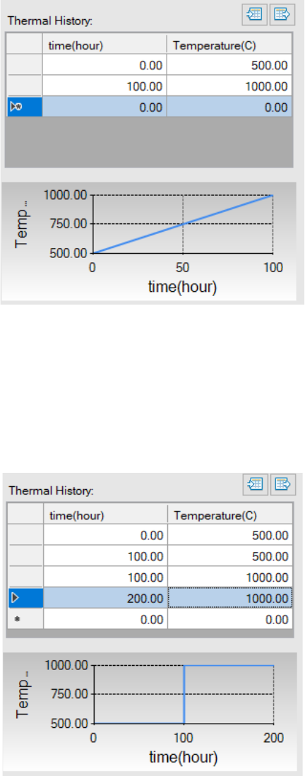
6.6.7 Set Thermal History
In the GUI of PanDiffusion, “Thermal History” controls temperature and the
duration at each temperature. The setting in Figure 6. indicates that the
temperature increases linearly from 500
o
C to 1000
o
C by 100 hours (5
o
C/hour).
193
Figure 6.21 A linear increment of temperature
The setting shown in Figure 6. means that the sample is held at 500
o
C for 100
hours, and then the furnace temperature is suddenly increased to 1000
o
C and
held there for another 100 hours.
Figure 6.22 A step-like thermal history.
6.6.8 Add Moments for Profile Outputs
For a calculation set up through GUI of PanDiffusion, two moments of profiles,
initial and final, will be provided by default. To add more intermediate
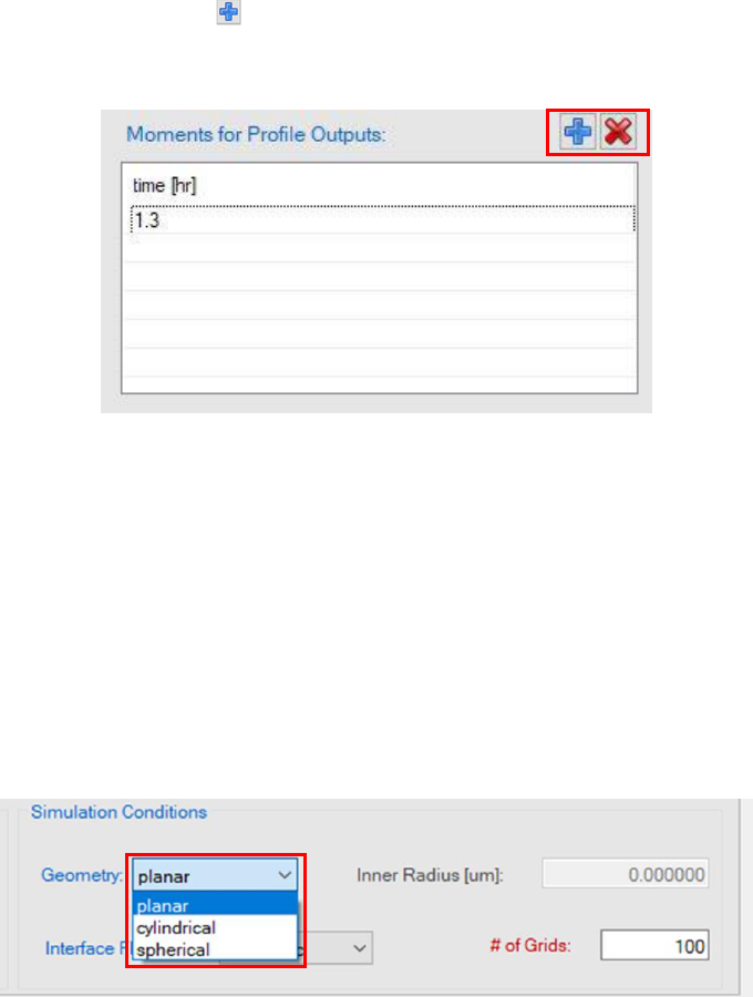
194
moments of profiles, click besides the “Moments for Profile Outputs”, and
edit time of the expected moment.
Figure 6.23 Add a moment for profile output at 1.3 hour.
6.6.9 Set Geometry
In the GUI of PanDiffusion, “Geometry” under “Simulation Conditions” decides
the shape of inter-grid interface. By default, “planar” is used for most diffusion
couple simulations. When particle homogenization or transformation is
performed, “spherical” or “cylindrical” could be selected depending on the
problem of interest.
Figure 6.24 Select the geometry
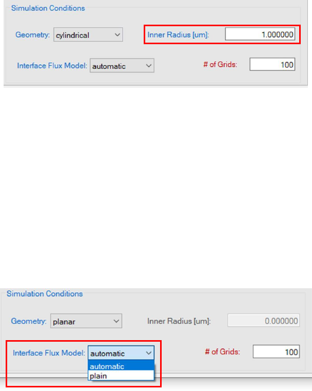
6.6.10 Set Inner Radius
When geometry other than “planar” is selected, user can set inner radius of cell,
to simulate for a tube or shell geometry. When “cylindrical” geometry is selected,
and the inner radius is non-zero, tube geometry is set up. When “spherical”
geometry is selected, and the inner radius is non-zero, shell geometry is set up.
195
Figure 6.25 Set Inner Radius
6.6.11 Set Interface Flux Model
In the GUI of PanDiffusion, “Interface Flux Model” under “Simulation
Conditions” decides how the grid composition evolves. When “automatic” is
selected by default, sharp interface between two distinct phases is calculated
with interface-fixed reference and local equilibrium applied at the interface.
When “plain” is selected, sharp interface between two distinct phases is
calculated in volume-fixed reference.
Figure 6.26 Select interface flux model
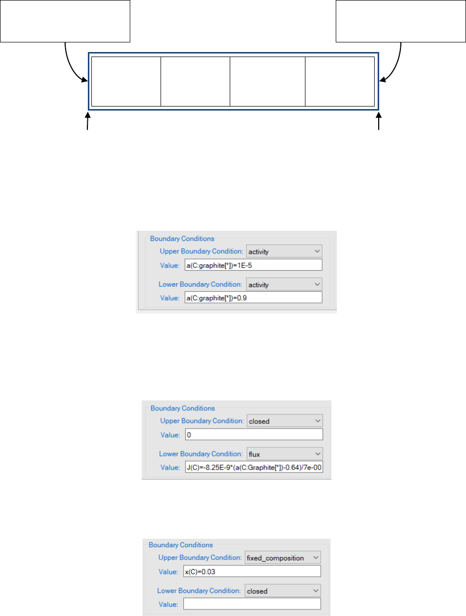
6.6.12 Set Boundary Conditions
There are “Upper Boundary Condition” and “Lower Boundary Condition” in
PanDiffusion. Their definitions are illustrated in the following figure:
196
Figure 6.27 Definition of boundary conditions
Fixed activity at boundaries can be set following the format:
Figure 6.29 Set fixed activity as a boundary condition
Mass flux expression at boundaries can be set following the format:
Figure 6.28 Set mass flux expression as a boundary condition
Fixed composition of boundaries can be set following the format:
Figure 6.29 Set fixed composition as a boundary condition
Region 1
Region 2
Region …
Region N
Simulation box
Left-hand side of
simulation box
Right-hand side of
simulation box
Lower Boundary
Condition
Upper Boundary
Condition
197
6.7 Settings in Dissolution Simulation
GUI
The features of general GUI for diffusion simulation have been demonstrated in
Section 6.6. In this section, we will present the features of the special GUI
for dissolution simulation.
Settings for units, number of grids, geometry, interface flux model, thermal
history and output profiles follow the same way as those in general GUI. The
phases are selected globally in dissolution GUI. There is no regional setting in
dissolution simulation. The global phase setting follows the same way as the
general GUI.
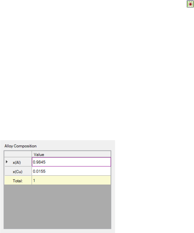
6.7.1 Set Alloy Composition
In the dissolution GUI, overall composition of an alloy is set in the following
section:
Figure 6.30 Alloy composition in dissolution simulation GUI.
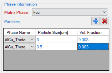
6.7.2 Set Matrix and Particle Information
Matrix phase and particle phases are explicitly selected in the “Phase
Information” section. There can be more than one particle phases. For each
particle phase, particle radius and volume fraction need to be set up.
198
Figure 6.31 Matrix and particle information in dissolution simulation.