
109
4 PanOptimizer
PanOptimizer is a module of Pandat
TM
software designed for optimizing
thermodynamic, kinetic and thermo-physical model parameters using
experimental data. The module allows users to develop their own databases or
model parameters for customized applications. This module is also easy to
master by students who want to learn thermodynamic modeling.
4.1 Features of PanOptimizer
Derived from the maximum likelihood principle, when the discrepancies
between model-calculated and experimental values are assumed to be
independent, identically distributed with a normal distribution function, a set
of model parameters with the best fit to the given experimental data can be
obtained by the least square method. In the real world the experimental data
may come from different sub-populations for which an independent estimate of
the error variance is available. In this case, a better estimate than the ordinary
least squares (OLS) can be obtained using weighted least squares (WLS), also
called generalized least squares (GLS), then the sum of the squares can be
written as
2
1
1
( ; , )
2
m
j j j j
j
w y x T c
=
−
(4.1)
The idea is to assign each observation a weight factor that reflects the
uncertainty of the measurement. According to our previous experiences this
method is efficient and reliable in the optimization of model parameters and
develop variety of databases.
4.2 PanOptimizer Functions
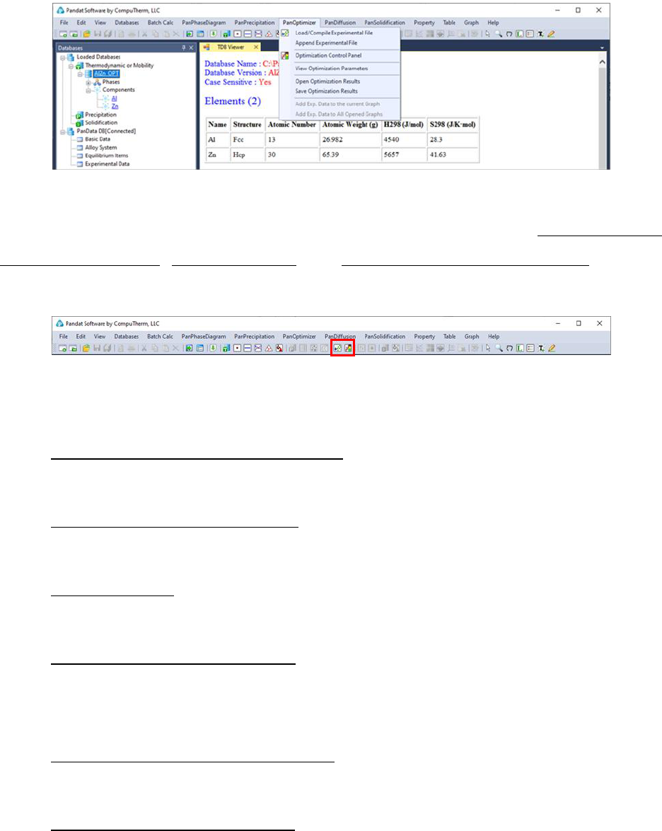
The major functions included in the PanOptimizer menu are shown in Figure
4.1:
110
Figure 4.1 The PanOptimizer Menu
The shortcut of the three commonly used functions Load/Compile
Experimental File, Rough Search and Optimization Control Panel are also
displayed in the Toolbar as shown in Figure 4.2.
Figure 4.2 PanOptimizer toolbar
The functionality of each function is given below:
➢ Load/Compile Experimental File: Load/Compile experimental data file
for model parameter optimization
➢ Append Experimental File: Append more experimental data from
different data file
➢ Rough Search: Global/Local search of initial values of model parameters
for obtaining the phase diagram topology of a system
➢ Optimization Control Panel: Allow user to set boundaries for the model
parameters to be optimized, select experimental data to be used, and
assign weight to each set of experimental data
➢ View Optimization Parameters: View/Edit model parameters to be
optimized
➢ Open Optimization Results: Open the saved intermediate optimization
results including the model parameters and experimental data

111
➢ Save Optimization Results: Save the intermediate optimization results
during the optimization process including the model parameters and
experimental data
4.3 Step by Step Instruction for
Optimization
In general, user should follow a few steps below to perform the model
parameter optimization.
4.3.1 Step 1: File preparation
4.3.1.1 Prepare the thermodynamic database file (.TDB)
In order to do the optimization, user must first define the model parameters to
be optimized in the thermodynamic database (.tdb). The model parameters to
be optimized can be defined in Pandat
TM
workspace where all the built-in
keywords are automatically highlighted. It can also be done through outside
text editor such as “Notepad”. Each model parameter that needs to be
optimized is defined by the keyword “Optimization”. The format of defining a
model parameter is:
Optimization [parameter name][low bound][initial value][high bound] N !
A definition sample for liquid phase in binary Al-Zn system is given as follows
$ Keyword Name Low Bound Init. Value High Bound
Optimization LIQ_AA 0 0; 60000 N !
Optimization LIQ_AAT -20 0; 20 N !
Optimization LIQ_BB -60000 0; 60000 N !
Optimization LIQ_BBT -20 0; 20 N !
Phase Liquid % 1 1 !
Constituent Liquid : Al, Zn : !
112
Optimization G(Liquid,Al;0) 298.15 G_Al_LIQUID; 6000 N !
Optimization G(Liquid,Zn;0) 298.15 G_Zn_LIQUID; 6000 N !
Optimization G(Liquid,Al,Zn;0) 298.15 LIQ_AA + LIQ_AAT*T; 6000 N !
Optimization G(Liquid,Al,Zn;1) 298.15 LIQ_BB + LIQ_BBT*T; 6000 N !
Two modes of optimization are allowed in the current version: one is “bounded”
optimization and the other one is “no bound” optimization. Even though the
low and high bounds will be in effect in the bounded optimization only, they
are required for definition of model parameters in a TDB file. The model
parameters can be named at users’ choices. It is suggested that the name is
related to the phase to be optimized. Note: User may use “%” to denote the
major species in a sublattice of a phase in a TDB file. PanOptimizer will
automatically assign the initial values for the major species denoted by “%”. The
following example means Zn is the major species in the first sublattice of the
Hcp phase:
Phase Hcp % 2 1 0.5 !
Constituent Hcp: Al, Zn%: Va:!
4.3.1.2 Prepare the experimental file (.POP)
Users need to provide their own experimental data file for optimization of model
parameters. The most widely accepted format for experimental data file in the
CALPHAD society is a POP file. PanOptimizer accepts most of the keywords in
the POP format and adds a few special keywords. In a POP file, a phase can
have four statuses: ENTERED, FIXED, DORMANT, and SUSPEND. The first
two statuses were used most frequently. When phases are in the ENTERED
status, PanOptimizer does not require user to input any initial values for
calculation since the truly stable phase equilibria will be found automatically
in this case with the built-in global optimization algorithm. On the other hand,
for those phases in FIXED or DORMANT status, the initial values should be
provided by the user. Example POP files are provided in the installation
dictionary of Pandat
TM
.
113
4.3.2 Step 2: Carry out optimization
Once above files have been prepared, user is ready to carry out optimization:
4.3.2.1 Load thermodynamic database file
First of all, the database file (.TDB) containing the phases to be modeled is
loaded by click the button. This database file defines the model type and
model parameters of each phase in the system. The model definition is
consistent with the currently accepted format in the CALPHAD society, and the
model parameters can be real numbers or variables to be optimized.
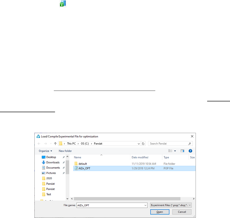
4.3.2.2 Load and compile experimental file
After loading a TDB file with defined model parameters to be optimized, users
should then load and compile the experimental POP file. Go to PanOptimizer
menu and choose Load/Compile Experimental File, user can then select the
POP file already prepared as shown in Figure 4.3. User can also choose Append
Experimental File to append new experimental data stored in a separate file to
the currently opened POP file.
Figure 4.3 Dialog window of loading an experimental file
114
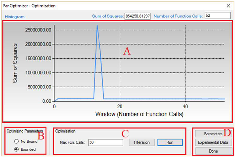
4.3.2.3 Perform Optimization
Once the TDB file and the experimental POP file are loaded, user is ready to do
the optimization. In the current version of PanOptimizer, the optimization is
controlled through the optimization control panel as shown in Figure 4.4.
There are four control areas in the optimization control panel. They are:
Histogram (A), Bound/Unbound Variables (B), Optimization (C), and
Optimization Results (D).
Figure 4.4 The optimization control panel.
4.3.2.4 Histogram (A)
Histogram is for displaying and tracing the history of the discrepancy between
model-calculated values and experimental data, which is characterized by the
Sum of Squares displayed during the whole optimization procedure. The
histogram plots the sum of squares vs. the number of function calls. The exact
value of the sum of squares in the current step can be found at the up-right
corner of this area.

115
4.3.2.5 Free Bound/Unbound Variables (B)
The user can choose the model parameters to be optimized in either the
bounded or the unbounded mode. In the bounded mode, the low and high
bounds defined in a TDB file will take into effects.
4.3.2.6 Optimization (C)
The goal of the optimization process is to obtain an optimal set of model
parameters so that the model calculated results can best fit the given
experimental measurements. The optimization process can be controlled by
choosing 1 Iteration or Run. With 1 Iteration, the maximum number of
function calls is set to be 2(N+2), where N is the number of model parameters
to be optimized. The user can click Run mode several times until the optimal
solution is found or the designated maximum number of function calls is
reached.
Here we take the binary Al-Zn system as an optimization example. The TDB and
POP files are available at the installing directory of Pandat
TM
“/Pandat_Examples/PanOptimizer/”. In this example, there are totally 11
parameters to be optimized and all the initial values are set to be zero. The
available experimental data include:
➢ mixing enthalpy of liquid phase at 953K
➢ invariant reaction at 655K: Liquid → Fcc + Hcp
➢ invariant reaction at 550K: Fcc#2 → Fcc#1 + Hcp
➢ tie-lines: Fcc#1+Fcc#2, Liquid + Fcc, Liquid + Hcp and Hcp + Fcc
Before the optimization, user may want to check the calculated results using
the initial set of model parameters without optimization. Phase diagram
calculation can be done through 2-D section calculation, and enthalpy
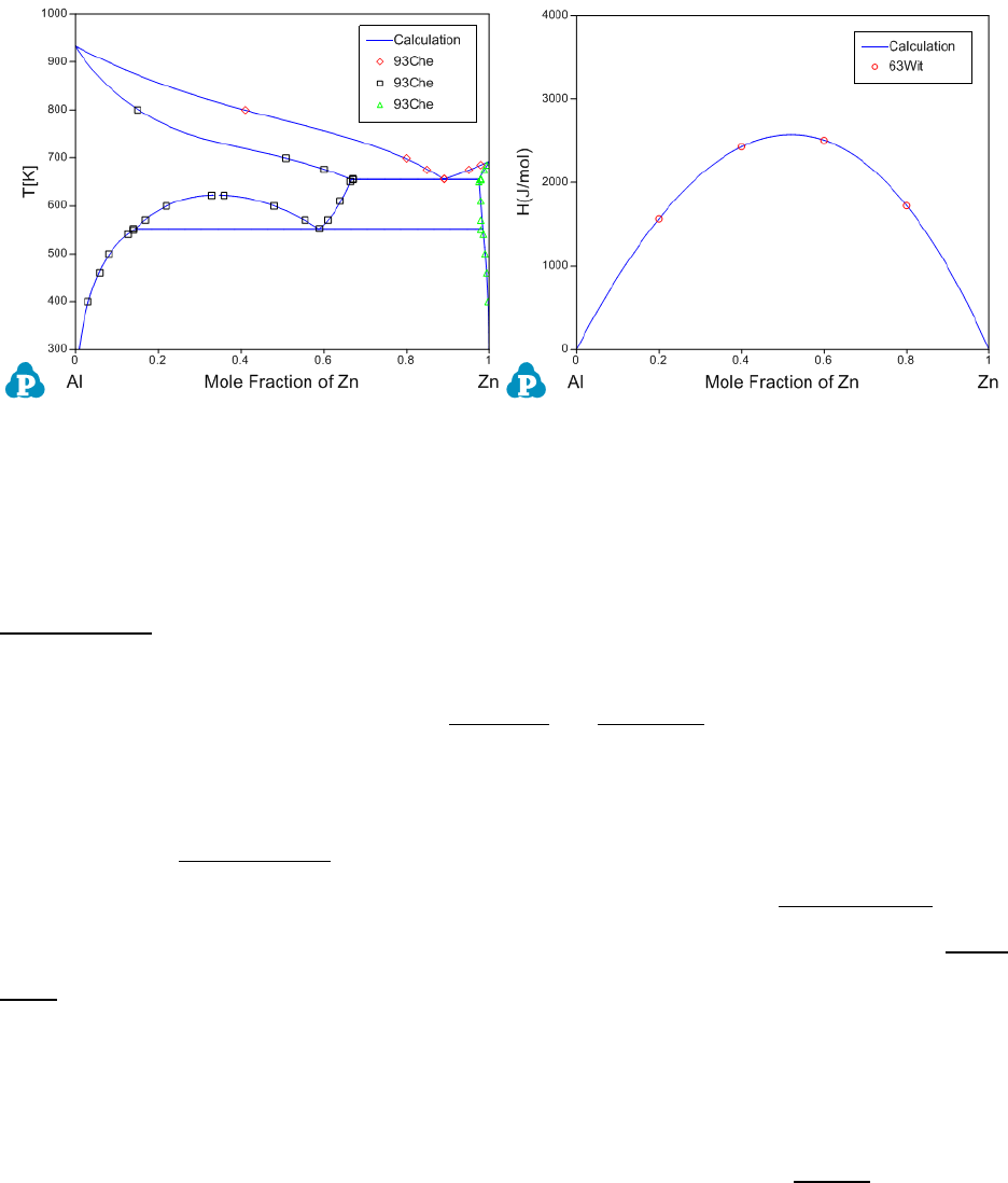
calculation can be done through the 1-D line calculation. Figure 4.5 shows the
calculated Al-Zn phase diagram and enthalpy of mixing for liquid phase at
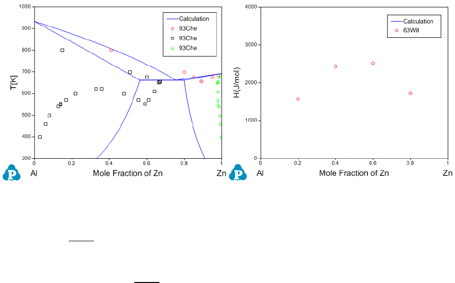
116
953K along with the given experimental data, respectively. The parameters
before optimization result in large discrepancies between the calculated values
and the experimental measurements. Optimization of these model parameters
(initially set as zero) is needed.
Figure 4.5 Comparisons between calculated results and experimental data
before the optimization
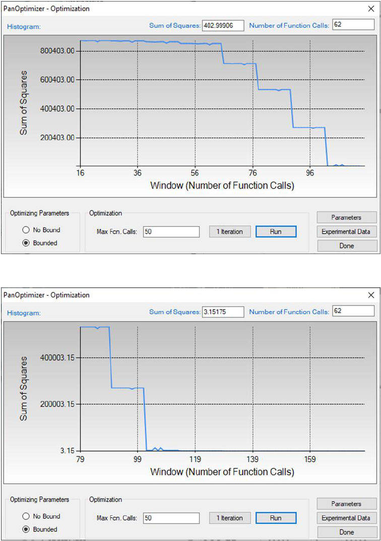
By clicking Run twice (two rounds), and each run performs 50 function calls,
the sum of squares decreases from 854251 to 403 as shown in Figure 4.6.
After another round of Run, the sum of squares decreases from 403 to 3.15 as
shown in Figure 4.7. Now, we can do the real time calculation using the
instantly obtained optimized parameters. The two comparisons in Figure 4.8
show excellent agreements between the calculated results and the measured
data. By selecting the command from PanOptimizer menu: PanOptimizer →
Add Exp. Data to the current Graph, user can add the corresponding
experimental data defined in the pop file directly to the calculated diagram for
comparison.
117
Figure 4.6 The sum of squares after two rounds of optimization
Figure 4.7 The sum of squares after another two rounds of optimization
118
Figure 4.8 Comparisons between the calculated results and the experimental
data after optimization
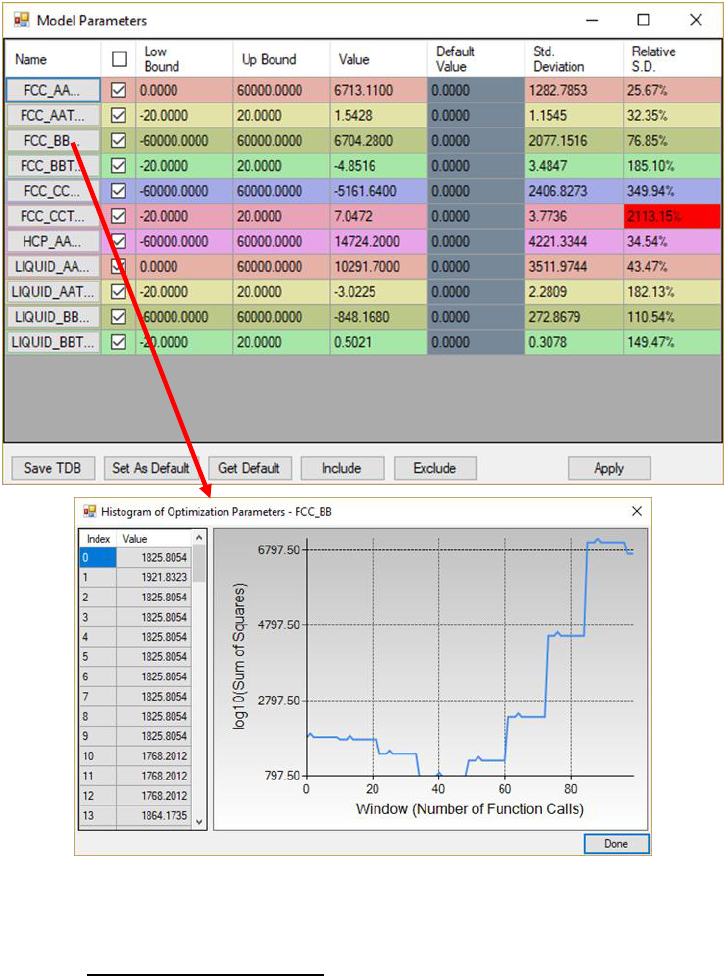
4.3.2.7 Optimization Results (D)
During optimization, user can check model parameters through the
Parameters button as shown in Figure 4.4. For each model parameter, user
can change its low bound, upper bound and initial value in the dialog window
as shown in Figure 4.9. User can Include or Exclude a certain parameter in
the optimization through the “check box” in front of the parameter. If a set of
optimized parameters is satisfactory, user can save this set of values as default
ones through Set Default shown in Figure 4.9. Otherwise, user can reject this
set of values and go back to previous default values through Get Default. User
also can save the TDB file with the optimized model parameters through Save
TDB. The standard deviation and relative standard deviation (RSD) of each
parameter are computed during optimization. The parameter evolution during
the last 100 iterations can be tracked by clicking the parameter name in the
table as indicated in Figure 4.9. It should be noted that any changes on model
parameters made by user will take into effect only after the “Apply” button is
clicked.
119
Figure 4.9 Dialog windows of Model Parameters and Histogram of Optimization
Parameters
By clicking the Experimental Data button on Figure 4.7, a table which lists
the calculated values together with the experimental data will pop out as
shown in Figure 4.10. This table allows user to view how well the current
optimized parameters describe each set of experimental data. If the discrepancy
is found to be large and not satisfied for a certain set of data, a larger weight
factor for this set of data can be given in the next round of optimization.
Through the column of “Residual” shown in Figure 4.10, user can see different
color after each comparison. The green means satisfactory results are achieved,
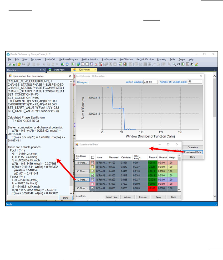
120
while the red color means large deviation remaining. Again, user can Include
or Exclude a certain experimental data set for the optimization through the
check box in front of each experimental data Name. Also, more detailed
experimental data information can be viewed by clicking the experimental data
ID in the table.
Figure 4.10 Dialog windows of Experimental Data and Optimization Item
Information
4.3.3 Step 3: Save/Open Optimization Results
During optimization, the user may save and load optimization file through Save
Optimization Results and Open Optimization Results (see Figure 4.11). The
optimization results file has the extension name of POR that can only be read
by PanOptimizer. Intermediate optimization results can be saved and restored
through these two operations. These functions are very useful especially when
a user is optimizing model parameters for a complicated system. The user can
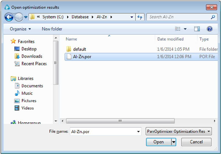
121
always go back to a certain middle stage and restart from there. This will save
user’s time by avoiding some repeated work.
Figure 4.11 Dialog window of open the saved optimization results
4.4 User-defined Property Optimization
The parameters for physical property, kinetic property, and user-defined
property can also be optimized with respect to experimental data just like the
parameters in a thermodynamic database. User can refer to section 8.4 for the
format to define user-defined property in a database. Similar to the
optimization of thermodynamic model parameters, user needs to define the
parameters to be optimized in the database and prepare a pop file with
corresponding experimental data. An example for the parameter definition in
the database is shown below.
$Thermal conductivity of pure element in the Fcc phase
PARAMETER ThCond(Fcc,Al;0) 298.15 +311.72511-0.09661*T-13510.26/T; 3000 N !
PARAMETER ThCond(Fcc,Cu;0) 298.15 +417.28065-0.06598*T+944.065/T; 3000 N !
122
$Thermal conductivity interaction parameters for Fcc phase to be optimized
OPTIMIZATION Fcc_TC 0 0; 60000 N !
OPTIMIZATION Fcc_TCT -50 -24.6; 0 N !
OPTIMIZATION Fcc_TC_1 -60000 0; 0 N !
OPTIMIZATION Fcc_TCT_1 0 28; 50 N !
PARAMETER ThCond(Fcc,Al,Cu;0) 298.15 +Fcc_TC+Fcc_TCT*T; 3000 N !
PARAMETER ThCond(Fcc,Al,Cu;1) 298.15 +Fcc_TC_1+Fcc_TCT_1*T; 3000 N !
And an example pop file for the experimental data is shown below.
$Thermal Conductivity of the Fcc phase at 1000K
TABLE_HEAD
CREATE_NEW_EQUILIBRIUM @@,1
CHANGE_STATUS PHASE * = S
CHANGE_STATUS PHASE Fcc = FIX 1
SET_CONDITION T=1000, P = P0, X(Fcc,Cu) = @1
EXPERIMENT ThCond(Fcc)= @3 : @4
TABLE_VALUES
$ x(Cu) x(Al) TC DTC
0.05 0.95 194 50
0.1 0.9 295 50
0.2 0.8 750 50
0.8 0.2 3116 50
0.9 0.1 2122 50
0.95 0.05 1343 50
TABLE_END
The optimization procedure is the same as that for thermodynamic parameters.
User may refer to the previous section for details and get the optimization
result step by step.