40
3 PanPhaseDiagram
3.1 Thermodynamic Database
PanPhaseDiagram is for phase diagram and thermodynamic property
calculation. Thermodynamic database is the prerequisite to fulfill such
calculations. A thermodynamic database represents a set of self-consistent
Gibbs-energy functions with optimized thermodynamic-model parameters for
all the phases in a system. The advantage of CALPHAD method is that the
separately-measured phase diagrams and thermodynamic properties can be
represented by a unique “thermodynamic description” of the materials system
in question. More importantly, on the basis of the known descriptions of the
constituent lower-order systems, the thermodynamic description for a higher-
order system can be obtained via an extrapolation method [1989Cho]. This
description enables us to calculate phase diagrams and thermodynamic
properties of multi-component systems that are experimentally unavailable.
In the following, thermodynamic models used to describe the disordered phase,
ordered intermetallic phase, and stoichiometric phase are presented. The
equations are given for a binary system, and they can be extrapolated to a
multi-component system using geometric models [1975Mug, 1989Cho].
The Gibbs energy of a binary disordered solution phase can be written as:
,
,,
ln ( )
ov
m i i i i A B v A B
i A B i A B v
G x G RT x x x x L x x
==
= + + −
(3.1)
where the first, second and third terms on the right hand of the equation
represent, respectively, the reference states, the entropy of ideal mixing, and
the excess Gibbs energy of mixing. Here x
i
is the mole fraction of a component i,
o
i
G
,
is the Gibbs energy of a pure component i, with an φ structure, R is the
gas constant, T is the absolute temperature, L
ν
is the interaction coefficient at
the polynomial series of the power ν. When ν = 0, it is a regular solution model,

41
and when ν = 0 and 1, it is a sub-regular solution model. Equation 3.1 can be
extrapolated into a multi-component system using geometric models, such as
the Muggianu model [1975Mug]. Ternary and higher-order interaction
parameters may be necessary to describe a multi-component solution phase.
An ordered intermetallic phase is described by a variety of sublattice models,
such as the compound-energy formalism [1979Ansara, 1988Ansara] and the
bond-energy model [1992Oates, 1995Chen]. In these models, the Gibbs energy
is a function of the sublattice species concentrations and temperature. The
Gibbs energy of a binary intermetallic phase, described by a two-sublattice
compound-energy formalism,
qp
BABA ),(:),(
, can be written as:
BABA
II
B
II
A
I
B
I
A
v
v
BAi
vII
B
II
A
II
B
II
A
BAi
I
i
v
v
jBA
vI
B
I
A
II
j
I
B
BAj
I
A
BAi
II
i
II
i
BAi
I
i
I
i
BAi BAj
ji
II
j
I
im
Lyyyy
LyyyyyLyyyyy
yy
qp
q
yy
qp
p
RTGyyG
,:,
,:
,
:,
,
,,, ,
:
)()(
]lnln[
+
−+−+
+
+
+
+=
==
=== =
(3.2)
where
I
i
y
and
II
i
y
are the species concentrations of a component,
i
, in the first
and second sublattices, respectively. The first term on the right hand of the
equation represents the reference state with the mechanical mixture of the
stable or hypothetical compounds: A,
qp
BA
,
qp
AB
, and B.
ji
G
:
is the Gibbs energy
of the stoichiometric compound,
qp
ji
, with an
structure. The value of
ji
G
:
can
be obtained experimentally if
qp
ji
is a stable compound; or it can be obtained
by ab initio calculation if
qp
ji
is a hypothetical compound. Sometimes,
ji
G
:
are
treated as model parameters to be obtained by optimization using the
experimental data related to this phase. The second term is the ideal mixing
Gibbs energy, which corresponds to the random mixing of species on the first
and second sublattices. The last three terms are the excess Gibbs energies of
mixing. The
""L
parameters in these terms are model parameters whose values
are obtained using the experimental phase-equilibrium data and
thermodynamic-property data. These parameters can be temperature

42
dependent. In this equation, a comma is used to separate species in the same
sublattice, whilst a colon is used to separate species belonging to different
sublattices. The compound-energy formalism can be applied to phases in a
multi-component system by considering the interactions from all the
constituent binaries. Additional ternary and higher-order interaction terms
may also be added to the excess Gibbs energy term.
For a reciprocal system with two sublattices, sometimes the interactions among
the two species on each sublattice are considered,
. The interaction
parameter is expressed as [2007Luk]
(3.3)
Pandat treats the term
as the interaction on the first sublattice
and the term
as the interaction on the second sublattice.
Pandat does not use the alphabetical order of species.
The Gibbs energy of a binary stoichiometric compound
pq
AB
,
m
G
, is described
as a function of temperature only:
,
()
m i i f p q
i
G x G G A B
= +
(3.4)
where
i
x
is the mole fraction of component i (i=p if it is A, and i=q if it is B), and
,
i
G
represents the Gibbs energy of component i with
structure;
()
f p q
G A B
,
which is normally a function of temperature, represents the Gibbs energy of
formation of the stoichiometric compound. If
()
f p q
G A B
is a linear function of
temperature:
( ) ( ) ( )
f p q f p q f p q
G A B H A B T S A B = −
(3.5)
then
()
f p q
H A B
, and
()
f p q
S A B
are the enthalpy and entropy of formation of the
stoichiometric compound, respectively. Equation (3.3) can be readily extended
to a multi-component stoichiometric compound phase.

43
The strategy of building a multi-component thermodynamic database starts
with deriving the Gibbs energy of each phase in the constituent binaries. There
are
2
n
C
constituent binaries in an n-component alloy system, where
)!(!
!
ini
n
C
i
n
−
=
(3.6)
To develop a reliable database, the Gibbs energies of these binaries must be
developed in a self-consistent manner and be compatible with each other.
Three binaries form a ternary, and a preliminary thermodynamic description
can be obtained by combining the three constituent binaries using geometric
models, such as the Muggianu model [1975Mug]. In some cases, a ternary
database developed in this way can describe a ternary system fairly well, while
in most cases, ternary interaction parameters are necessary to better describe
the ternary system. If a new phase appears in the ternary, which is not in any
of the constituent binaries, a thermodynamic model is selected for this ternary
phase, and its model parameters are optimized using the experimental
information for this ternary phase. There are a total of
3
n
C
ternary systems in
an n-component system. After thermodynamic descriptions of all
3
n
C
ternaries
for an n-component system are established, the model parameters are simply
used to describe quaternary and higher-order systems using an extrapolation
approach. High-order interaction parameters are usually not necessary
because although interactions between binary components are strong, in
ternary systems they become weaker, and in higher-ordered systems they
become negligibly weak [1997Kattner, 2004Chang]. It is worth noting that the
term, “thermodynamic database” or simply “database”, is usually used in the
industrial community instead of “thermodynamic description”, particularly for
multi-component systems.
At CompuTherm, multi-component databases have been developed for variety
of alloys, such as for Al-alloys, Co-alloys, Cu-alloys, Fe-alloys, Mg-alloys, Mo-
alloys, Nb-alloys, Ni-alloys, Ti-alloys, TiAl-alloys, high entropy alloys, and
44
solder alloys. Information for these databases is available in the
“Thermodynamic Database User’s Guide” from CompuTherm.
3.2 Thermodynamic Calculation
3.2.1 Load Database
Pandat
TM
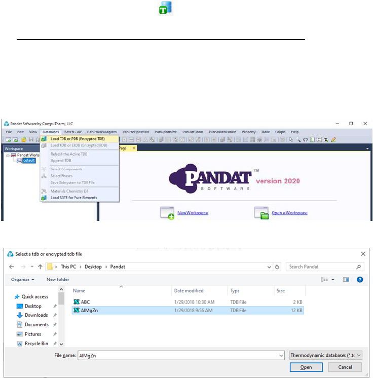
can load both PDB and TDB database files. This command can be
accessed through the toolbar icon . User can also load a database file using
the Menus Database→Load TDB or PDB (Encrypted TDB) as shown in Figure
3.1. Select a database file from hard drive and click open button, or just double
click the database file. Users can store the databases in any directory in the
computer.
Figure 3.1 Load a database from hard drive through Menus
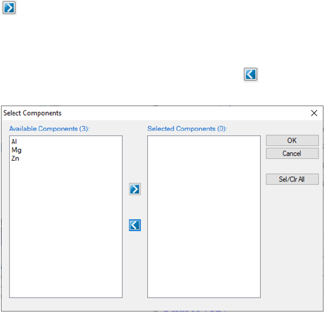
Immediately after a database is successfully loaded, a popup window shown in
Figure 3.2 will ask the user to select the components for subsequent
calculations. To add a component to the list of selected components, click on
the component on the list of Available Components on the left column, and
45
click on the button to send them to the Selected Components on the right
column. To select several components at one time, hold the <Ctrl> key and use
mouse to select multiple components. To remove a component from selected
components list, use mouse to select it, and click the button.
Figure 3.2 Select components for further calculation
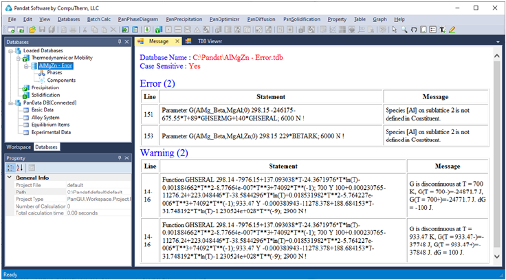
While loading a database file, Pandat
TM
checks the self-consistency of the
database. A message will be displayed if the database is not internally
consistent such as duplicated definitions of a function, missing definition of
components or species in a sublattice, and so on. There are two types of
messages: Error and Warning, as shown in Figure 3.3. The warning message
can be ignored but the errors must be fixed, otherwise the database cannot be
loaded. It is recommended to correct both error and warning before performing
calculation. If you have difficulties loading a particular TDB or PDB file, please
contact CompuTherm, LLC, and we will help resolve the problem.
46
Figure 3.3 A typical message when loading a database
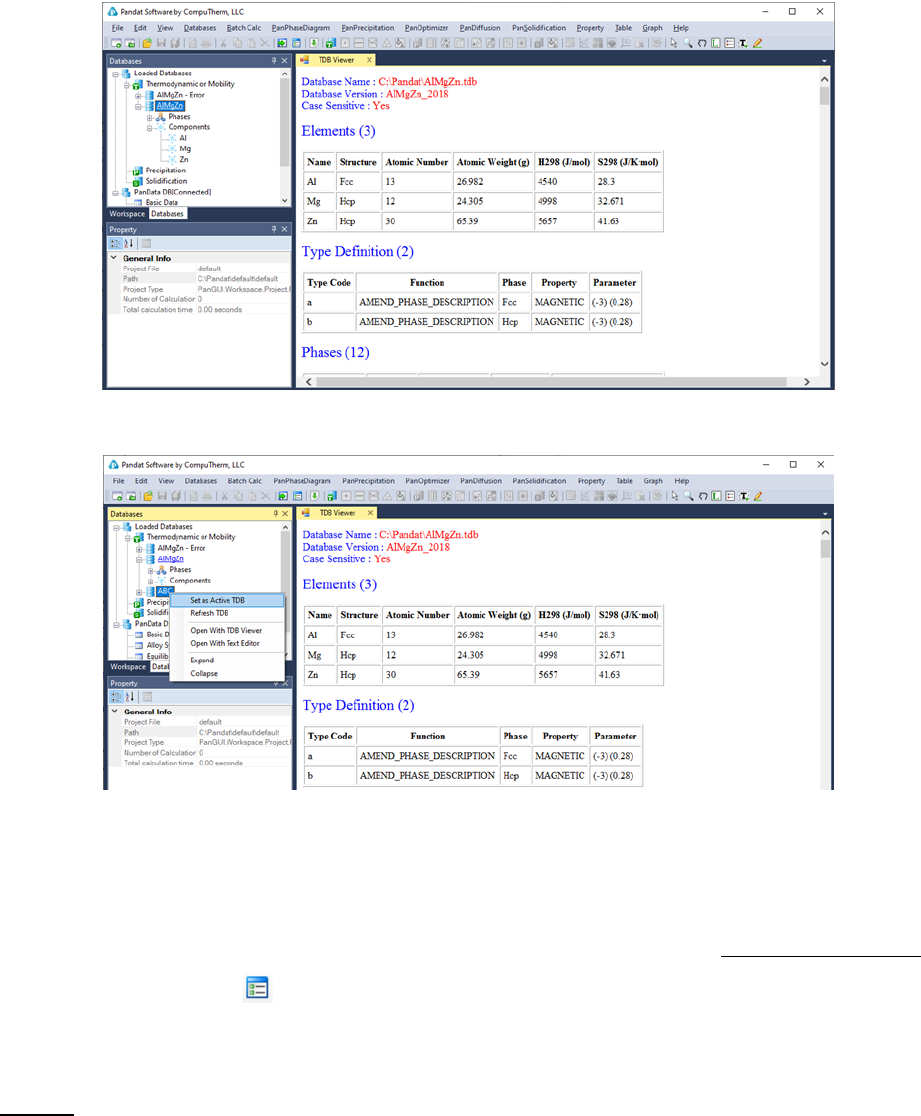
The successfully loaded database will be automatically summarized in the TDB
Viewer mode in the main Display window as shown in Figure 3.4. For a TDB
format database, the summary includes elements, type definitions, phases with
name and thermodynamic model, model parameters and defined functions. For
a PDB format database, the model parameters and functions will not be
displayed. The user can open a TDB format database with the Text Editor mode
by right click of the mouse on the database name in the explorer window. The
Text Editor is actually a built-in notepad for text files. User can use the Text
Editor directly within Pandat
TM
workspace to edit the TDB database, or he/she
can always use his/her favorite text editor to do it.
Multiple databases can be loaded into the same workspace but only one is
activated. The current calculation will use the activated database, which is
highlighted in the explorer window at Database view. The user may set the
inactive database to be active with right click of the mouse as shown in Figure
3.5.
47
Figure 3.4 The TDB viewer mode for database summary
Figure 3.5 Set an inactive database to be active
3.2.2 Options
To configure the calculation options, go through the menus (View → Options),
or click on the icon on the toolbar. A pop-up dialog box allows the user to
change the units, and output formats of default Table and Graph.
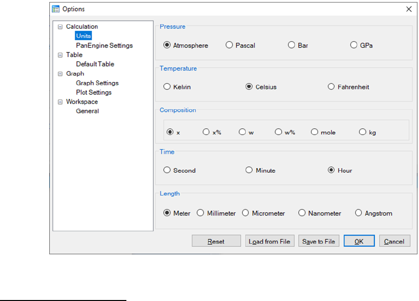
Units: This dialog box allows the user to choose the units to be used in the
calculation. Use the mouse left button to select a proper unit for each property
and click “OK” to complete the unit setting as shown in Figure 3.6.
48
Figure 3.6 Set units for a calculation in Options
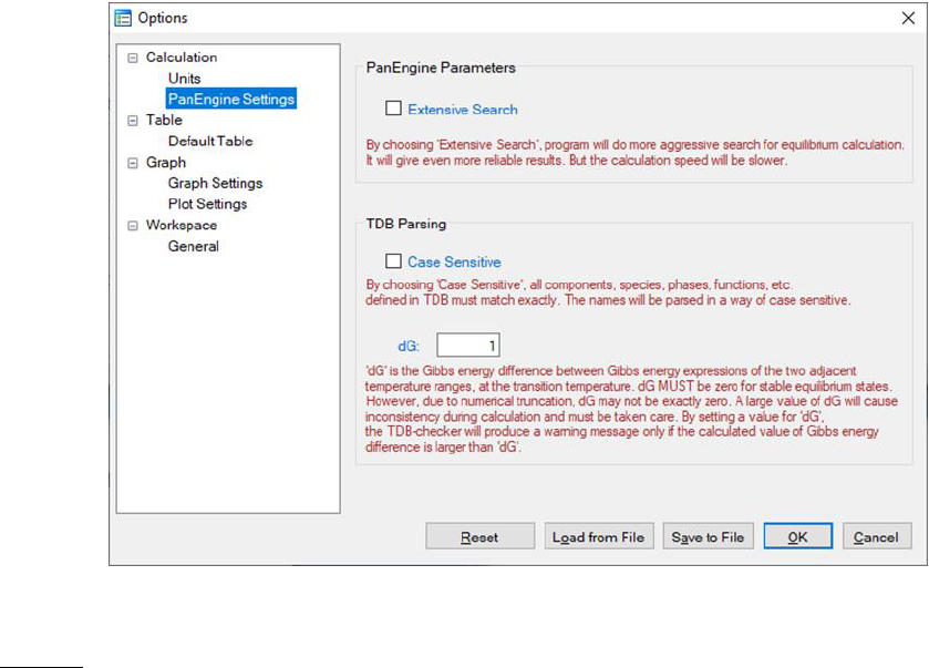
PanEngine Settings: This dialog box allows the user to change the PanEngine
Parameter and TDB Parsing parameters as shown in Figure 3.7. When
“Extensive Search” is checked, PanEngine will perform a more thorough search
of the global equilibrium state in case the Normal Search missed it. For
majority of cases Extensive Search is not necessary and will give the same
answer as that of Normal Search. The calculation will take longer time when
Extensive Search is chosen. Extensive Search is recommended only when the
user found metastable equilibrium in a particular calculation.
If the “Case Sensitive” box is checked, all the components, species, phases,
functions, etc. defined in the TDB will be parsed in a way of case sensitive and
should match exactly, in other words, the uppercase letters are treated as
different from the corresponding lowercase letters.
The Gibbs energy of a pure component with a certain crystal structure is
usually segmental function of temperature and is represented by different
Gibbs energy expression at different temperature range. dG represents the
Gibbs energy difference obtained from the two Gibbs energy expressions at
49
adjacent temperature ranges at the transition temperature. Ideally, dG is zero if
the two Gibbs energy expressions give the exact same value at the transition
temperature. However, due to numerical truncation, dG is usually not zero.
The default setting of dG in PanEngine is 1.0 J/mole atom. A warning message
will be sent to TDB viewer if dG is greater than 1.0. A large dG will cause
calculation fail, therefore should be fixed in the TDB file. User can set this
value to a bigger or smaller value according to his/her tolerance.
Figure 3.7 PanEngine Settings in Options
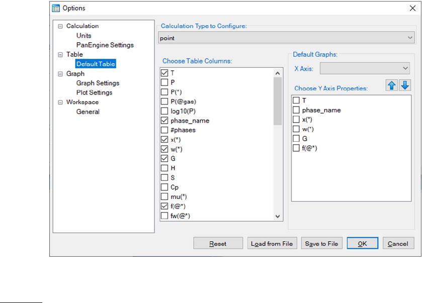
Table: This dialog box allows a user to customize the default output table with
the properties the user needs. As shown in Figure 3.8, user first needs to
choose the “Calculation Type to Configure” which includes point, line, section,
solidification and so on. Once the Calculation Type is selected, all the possible
properties for the chosen Calculation Type will be listed in the “Choose Table
Columns”. The user can check the box in front of each item to select the
column to be shown in the default output table. All the selected properties will
be listed in the “Choose Y Axis Properties”. In this same dialog, user can also
50
define the X axis and Y axis of the default graph that is automatically shown
when a calculation finishes.
Figure 3.8 Set default table output and default dataset for graph output
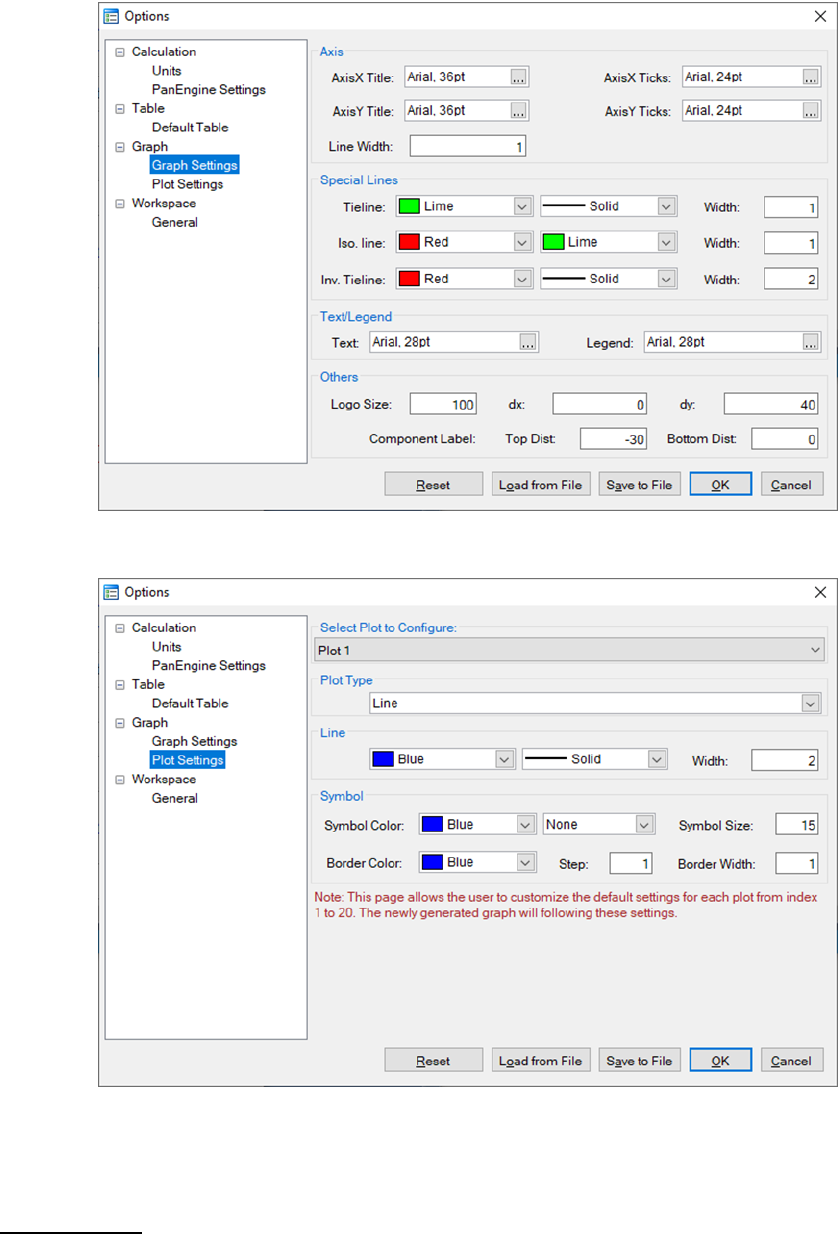
Graph: This dialog box allows the user to set up the appearance of the output
graph. As shown in Figure 3.9, user can set the font and size of the texts, color
and width of the lines, color, shape and size of the symbols, and logo size and
positions for the default graph. User can also set the color and width of the
lines, color, shape and size of the symbols for different plots in one graph as
shown in Figure 3.10.
52
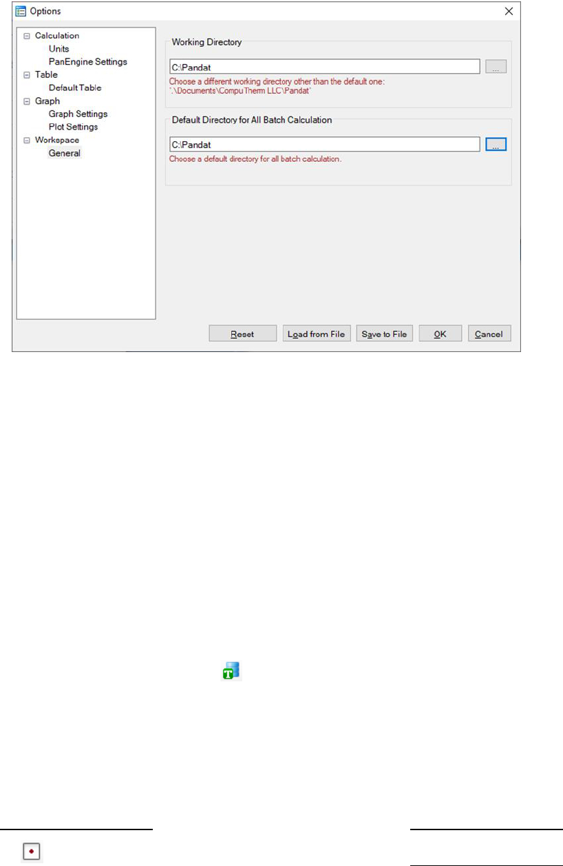
Figure 3.11 set up the default working directory for Pandat workspace
It should be pointed out that “Options” gives users the opportunity to change
the PanEngine Setting and customize the output of Default Table and Graph.
However, users do not have to do anything if not necessary. By default, the
most popular setting has been selected for each type of calculation.
3.3 Tutorial
The Al-Mg-Zn is used as an example for the following calculations.
TheAlMgZn.tdb is in the PanPhaseDiagram directory under Pandat
TM
examples.
Load the database by clicking the button and select all three components.
3.3.1 Point Calculation (0D)
This function allows the user to calculate the stable phase equilibrium at a
single point in a multicomponent system.
Go to PanPhaseDiagram on the menu bar and select Point Calculation or
click the button on the tool bar. The dialog box for Point Calculation as

53
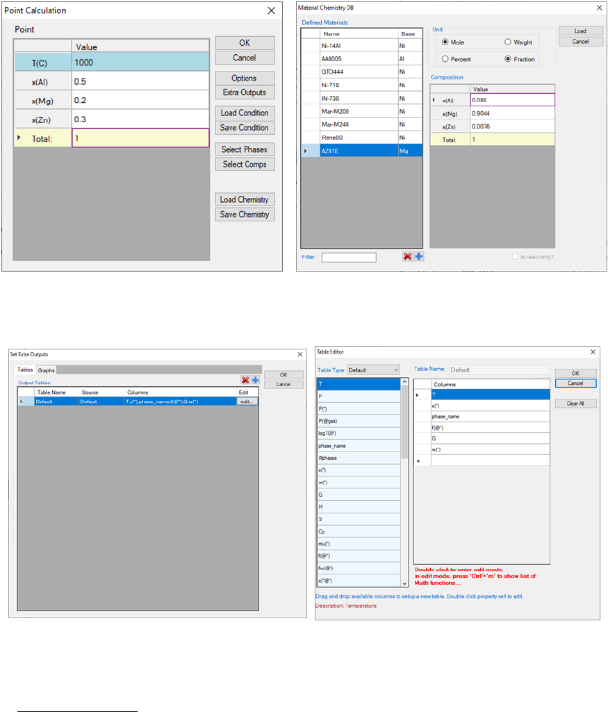
shown in Figure 3.12(a) allows the user to set up the calculation conditions:
composition and temperature. User can either input the conditions manually
or use the Load Condition function to load from an existing batch file. User
can always save the current calculation condition to a batch file by clicking the
Save Condition button, or save the alloy composition on hard disc by clicking
Save Chemistry button. User can load the alloy composition for the future
calculation using the function Load Chemistry following Figure 3.12(b).
The functions of other buttons as shown in Figure 3.12(a) are given below. User
can access the Options window again by clicking Options and make changes
for the units. Please refer to the previous section for information on the
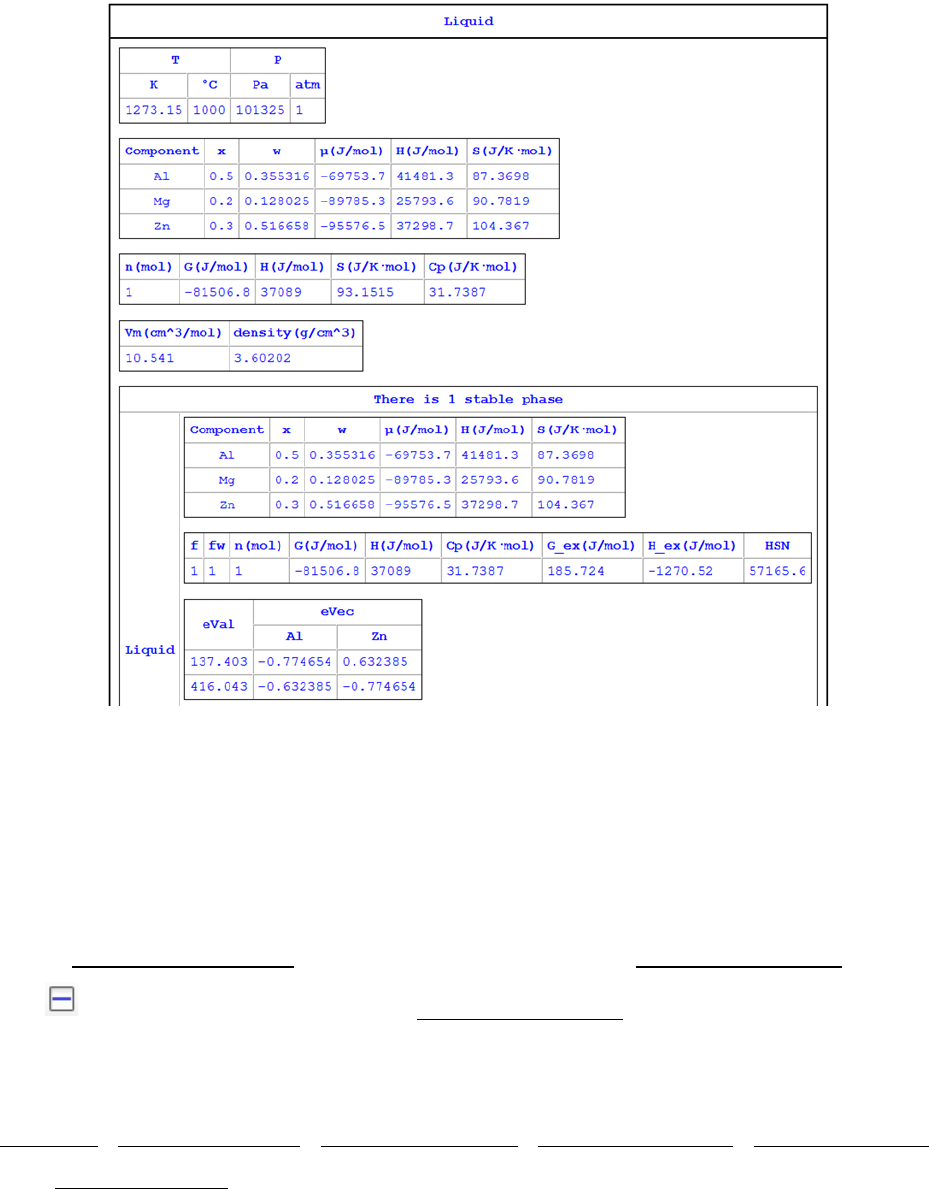
Options window. The Extra Outputs button allows the user to modify the
default output table and graph and add more tables and graphs as needed. A
pop out window as shown in Figure 3.13(a) provides the access to the table and
graph for output. User may add or delete output table/graph using the buttons
and , or modify the selected table/graph by clicking the “edit…” button.
Please refer to the previous section for information on Table Edit. The Graph
dialog is slightly different from that described in the previous section. As shown
in Figure 3.13(b), data source for the graph can only be the tables generated
from the calculations and there is a check box for the triangle plot. The
operations for editing the graph are the same as those described in the
previous section.
54
(a) (b)
Figure 3.12 Set alloy composition and Temperature for point calculation
(a) (b)
Figure 3.13 Set extra output table for point calculation
The Select Phases button in Figure 3.12(a) leads the user to a dialog which
allows the user to select or deselect phases to be involved in the calculation as
shown in Figure 3.14. The default setting is that all the phases in the system
are selected and listed in the Entered Phases column, which means all the
phases are involved in the equilibrium calculation. User can select the phases
that will not participate in the equilibrium calculation by sending them to the
Dormant Phases or Suspended Phases column using mouse to drag and drop

55
or using the button. To select several phases at one time, hold the <Ctrl>
key and use mouse to select multiple phases. The Suspended Phases means
that the phases in that column are excluded in any calculations. The Dormant
Phases means that the phases in that column are excluded from the
equilibrium calculation but will be included for the property calculations, such
as driving force, after the equilibrium calculation is finished. The Dormant
Phases option mainly works for point calculation and line calculation. The
Suspended Phases option is usually used for metastable phase equilibrium
calculations.
Figure 3.14 Select Phases dialog
The Select Comps button in Figure 3.12(a) allows user to make last minute
change on the component selection. Please refer to the previous section for
information on the Select Components window.
After the calculation is completed, the calculated results are displayed in the
Pandat
TM
main display window as shown in Figure 3.15. The listed properties
include thermodynamic properties at this point, such as Gibbs energy,
enthalpy, entropy and heat capacity. It also lists the stable phases and the
fraction of each phase.
56
Figure 3.15 Results of point calculation
3.3.2 Line Calculation (1D)
This function allows the user to perform a series of point calculations along a
line in a multicomponent system.
Go to PanPhaseDiagram on the menu bar and select Line Calculation or click
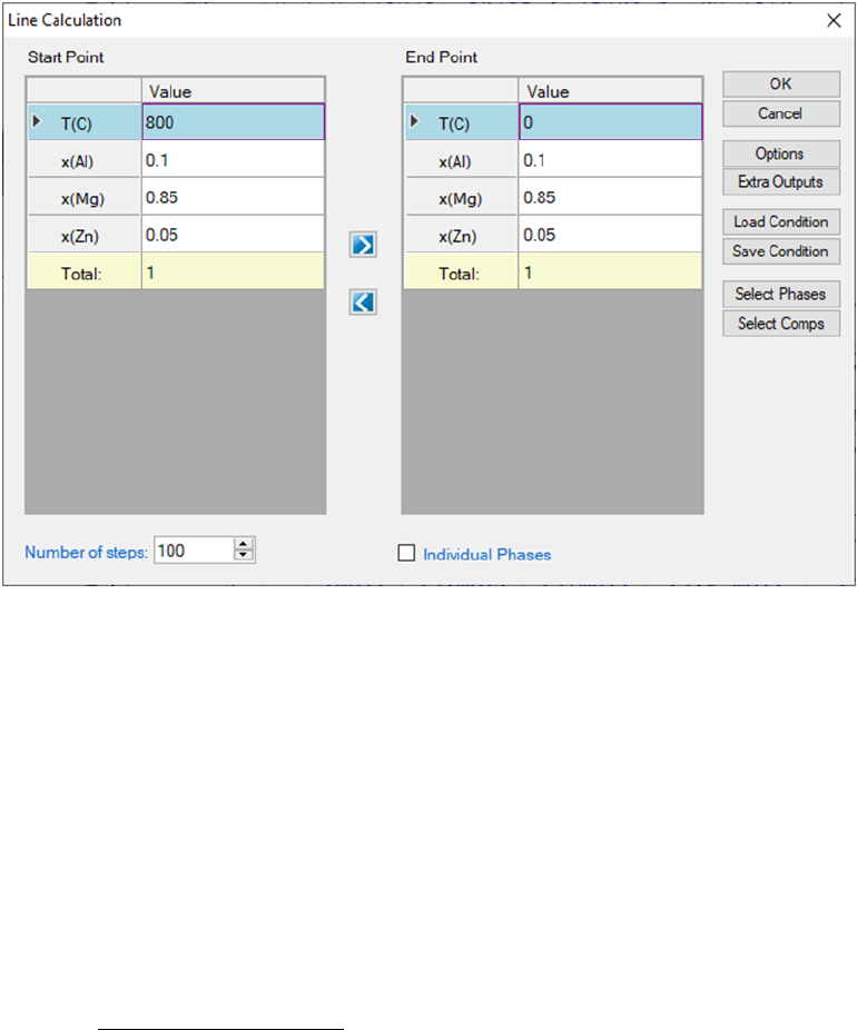
the button on the tool bar. The Line Calculation (1D) dialog box allows the
user to set the start and end points of the line, and the number of steps to
calculate along the line as shown in Figure 3.16. User can also access the
Options, Extra Outputs, Load Condition, Save Condition, Select Phases,
and Select Comps the same way as those in point calculation. Note that the
line calculation set up in Figure 3.16 is along the line of fixing alloy chemistry
with varying temperature.
57
Figure 3.16 Set calculation conditions for a line calculation
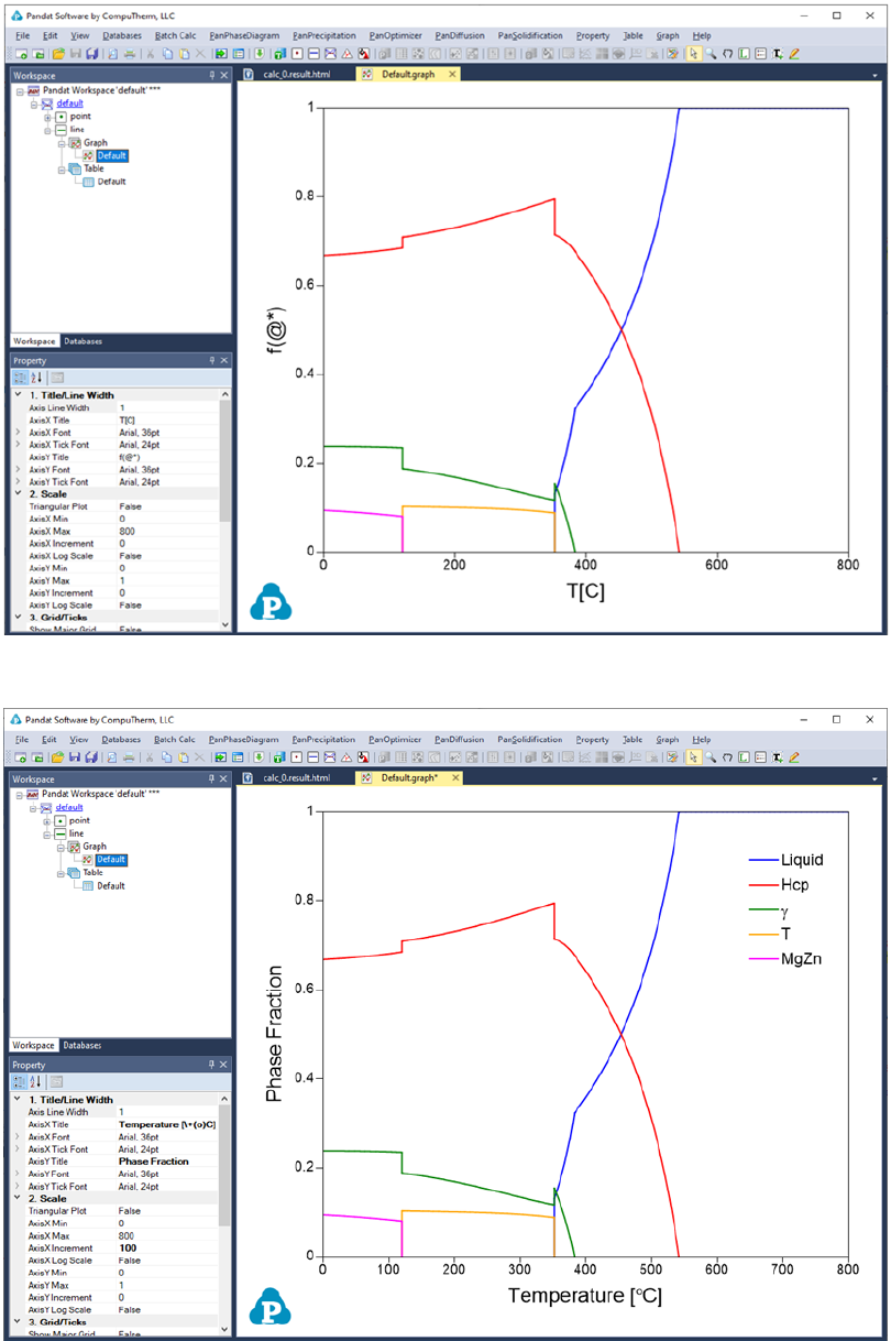
The calculated results are stored in both graph and table. The default graph
plots the variation of fraction of each phase with respect to temperature, as
shown in Figure 3.17. User can modify the graph through the Property window
by modifying the title, scale and add legend to get a better view as shown in
Figure 3.18. In the Explore window, user can double click the “Default” under
the “Table” tree to view the default table. User can select any columns to create
new plots. Furthermore, select the “Table” and right click the mouse, user has
the option to Add a New Table to generate new tables and then plot other
figures as needed.
58
Figure 3.17 Default graph view of the line calculation result
Figure 3.18 Modify the graph with a better view
59
It should be pointed out that user can certainly choose to fix the temperature
and vary the alloy composition for a line calculation.
3.3.3 Section Calculation (2D)
This function allows user to calculate any two-dimensional section of a
multicomponent system. Three non-collinear points in the calculation space
are required to define a 2D section. Common 2D section diagrams are
isotherms and isopleths.
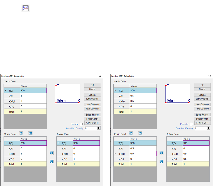
Go to PanPhaseDiagram on the menu bar and select Section Calculation or
click the button on the tool bar. The Section (2D) Calculation dialog box
allows the user to set up the calculation conditions in terms of composition
and temperature. Figure 3.19 shows the two most common 2D calculations for
a ternary system: (a) Isotherm which is a horizontal section that fixes the
temperature and (b) Isopleth which is a vertical section that uses the
temperature as the Y axis.
(a) (b)
Figure 3.19 Set calculation conditions for section calculation
60
The composition at each point should be self-consistent. For example,
x(Al)+x(Mg)+x(Zn)=1 for the Al-Mg-Zn ternary system. It is not necessary to have
a correlation between the Y-Axis point, the Origin point and the X-Axis point.
User can also access the Options, Extra Outputs, Load Condition, Save
Condition, Select Phases, and Select Comps windows through this dialog box.
The Contour Lines option allows the user to add special lines to the output
results, such as Tc curve and T
0
curve as shown in Figure 3.20.
Figure 3.20 Contour Lines dialog
The setting on Figure 3.19(a) defines a calculation of an isothermal section for
the Al-Mg-Zn ternary system at 300
o
C. The setting on Figure 3.19(b) defines a
vertical section calculation from the middle of the Al-Mg binary to the middle of
the Mg-Zn binary in the temperature range of 300-800
o
C. The results from a
Section calculation are displayed in two types of format in the Pandat
TM
main
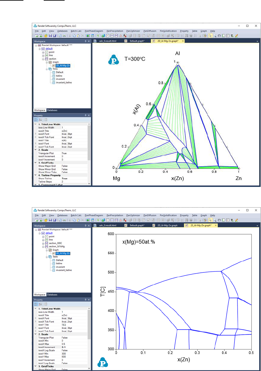
window: Graph and Table. Figure 3.21 and Figure 3.22 show the graph view of
the calculation results for the settings in Figure 3.19 (a) and (b), respectively.
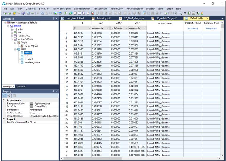
Figure 3.23 shows a table view of the isotherm calculation result. User can
switch between Graph view and Table View by double clicking on the graph
name or table name in the Pandat
TM
Explore window. Other operations on
61
Graph and Table, such as labeling and adding a legend, have been discussed
in details in Section 2.3 and Section 2.4.
Figure 3.21 Isothermal section of the Al-Mg-Zn ternary system at 300
o
C
Figure 3.22 Isopleth of the Al-Mg-Zn ternary system at 50 at.% of Mg
62
Figure 3.23 Table view for the 300
o
C isotherm calculation results
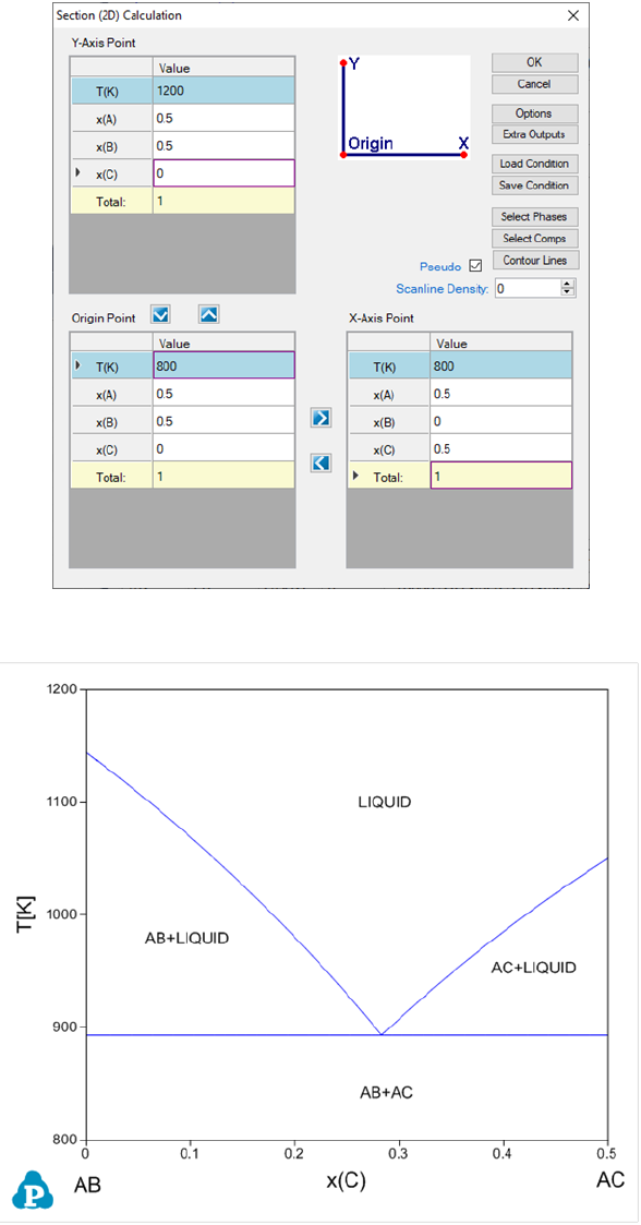
3.3.4 Pseudo Binary Section
Sometimes a ternary isoplethal section is so special that all the tie-lines are
with this section to form a pseudo binary section. To calculate this type of
section, a special algorithm is designed in Pandat
TM
and a special keyword
“pseudo” is required. In the folder where Pandat
TM
software is installed: Pandat
2020 Examples/PanPhaseDiagram/Pseudo_Binary/, there is an example A-
B-C system with “Pseudo_Binary.tdb”. After load the database file, click on
“Section Calculation”. Set the calculation condition and check the “Pseudo”
box, as shown in Figure 3.24. The calculated pseudo binary section is shown in
Figure 3.25.
63
Figure 3.24 Set calculation condition for a pseudo-binary section
Figure 3.25 A pseudo-binary section in a ternary A-B-C system
64
3.3.5 Contour Diagram
Contour diagram shows how a property changes in a 2D or 3D diagram
[2015Che]. The most commonly used contour diagram is the ternary
isothermal lines superimposed on a liquidus projection. Another example is the
activity contour diagram. Pandat
TM
extends contour diagram to many other
properties including thermodynamic properties, physical properties and any
combination of them. In the following, we will give a few examples of useful
contour diagrams. Please keep in mind that Pandat
TM
can plot many other
contour diagrams beyond these examples.
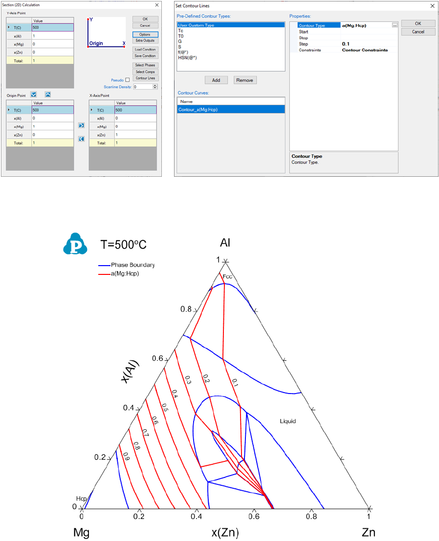
3.3.5.1 Activity Contour Diagram
Let’s use the contour diagram of Mg activity in Al-Mg-Zn as the first example.
Figure 3.26(a) shows the input window for calculating the isothermal section of
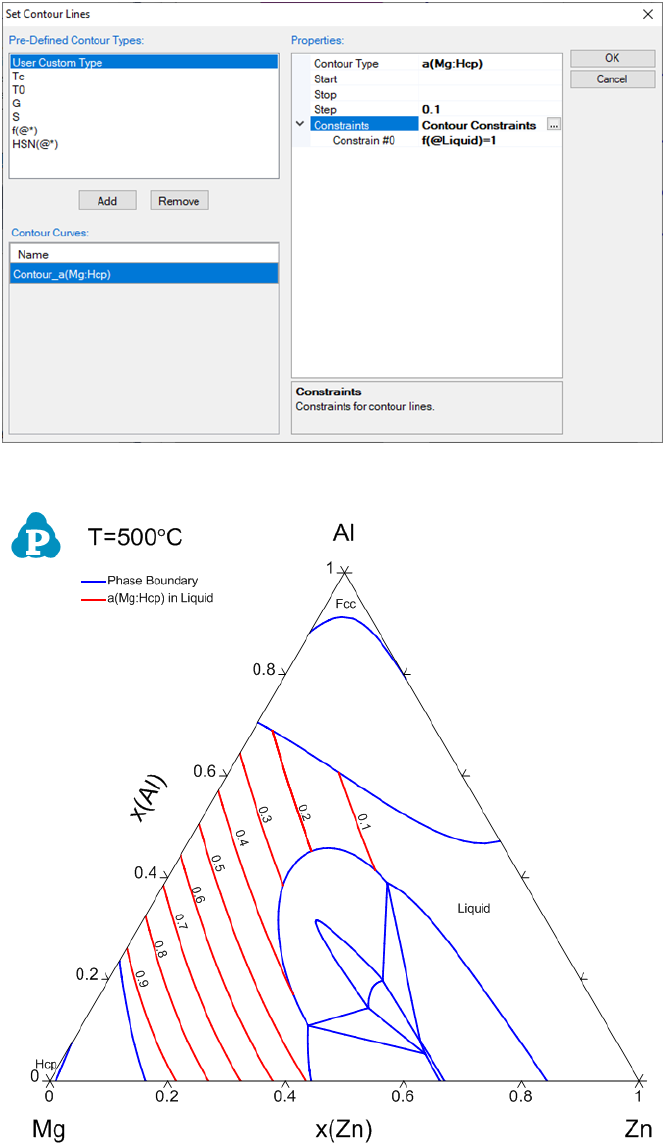
Al-Mg-Zn at 500°C. In this input window, there is a button “Contour Lines”.
Click on the “Contour Lines” button, a new window “Set Contour Lines” will
pop out, as shown in Figure 3.26(b). Click on “Add” button and change the
“Contour Type” to “a(Mg:Hcp)”, which means that the contour diagram is for
the activity of Mg with reference state of Hcp. There are three initials related to
which values of the contour lines to be calculated: “Start”, “Stop” and “Step”. In
this example, “Start” and “Stop” can be left as empty and Pandat
TM
will search
for all possible values. User can set values for “Start” and “Stop” for specific
range of the contour lines. However, the value of “Step” must be given. Another
condition “Constraints” will be explained later. Figure 3.26(b) sets the initial
condition to calculate the contour lines for the activity of Mg referring to Mg in
Hcp phase with the step size of 0.1. Click “OK” in this window and also in the
“Section (2D) Calculation” window to proceed the calculation. The calculated
isothermal diagram with the contour lines of activity of Mg is shown in Figure
3.27 after labeling.
65
(a) 2D Diagram input window (b) Contour Diagram input window
Figure 3.26 Input windows for contour diagram of activity of Mg at 500°C
Figure 3.27 Contour diagram of activity of Mg in the isothermal section of Al-
Mg-Zn at 500°C
If we want to calculate the contour lines of the Mg activity only in the liquid
phase, it can be achieved by setting a constraint in the contour diagram input
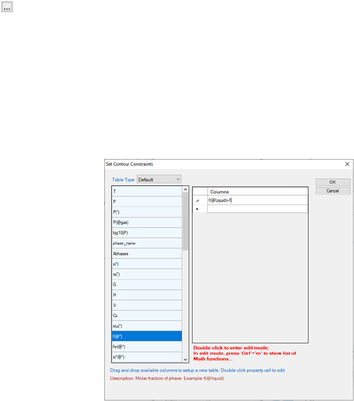
66
condition. In Figure 3.26(b), click on “Contour Constraints”, a small button
will show up. Click on it, we will have a window of “Set Contour
Constraints” as shown in Figure 3.29. Add “f(@Liquid)=1” as the constraint
in this window and then click “OK” to return to “Set Contour Lines” window
as in Figure 3.29. This will set a constraint on the contour line calculation that
only the contour lines with “f(@Liquid)=1” will be calculated. Figure 3.30 is
the calculated phase diagram with the contour diagram of a(Mg) only in the
liquid phase region in the isothermal section of Al-Mg-Zn at 500°C.
Figure 3.28 Set contour constraints window
67
Figure 3.29 Input windows for setting constraints for the contour diagram
Figure 3.30 Contour diagram of activity of Mg only in liquid phase in the
isothermal section of Al-Mg-Zn at 500°C
68
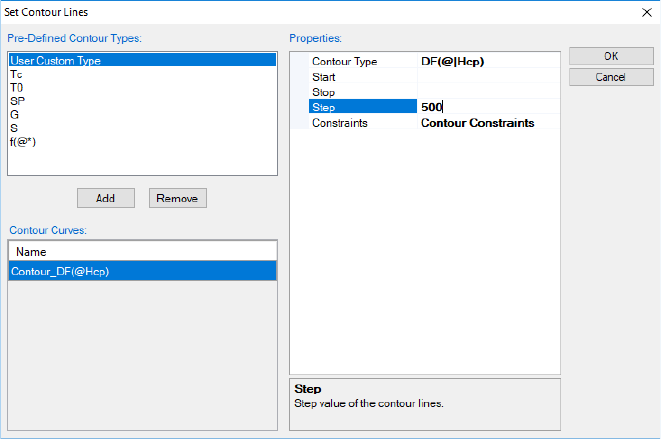
3.3.5.2 Driving Force Contour Diagram
Contour diagram is also useful in viewing the stability of a phase comparing to
the equilibrium state. Figure 3.31 shows the driving force contour lines of the
Hcp phase in the Al-Mg-Zn system at 500°C. The contour type is defined as
DF(@|Hcp)as shown in Figure 3.31 (see Table 2.2 for the definition of DF).
Since Hcp phase may not be stable in all the phase regions in this isothermal
section, in between “@” and “Hcp” a vertical bar symbol “|” is added to specify
that the phase Hcp is in the “entered” status. From Figure 3.32, we see that
Hcp phase has less driving force to be stable in the central region of the
compositional triangle.
Figure 3.31 Set driving force contour
69
Figure 3.32 Contour diagram of the driving force of the Hcp phase relative to
the equilibrium phases in Al-Mg-Zn at 500°C
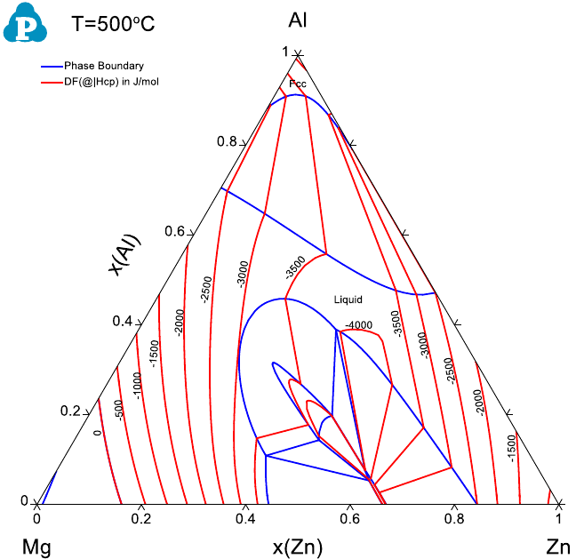
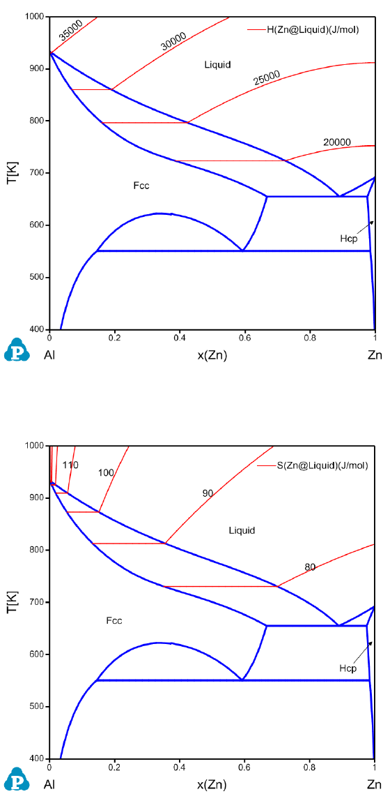
3.3.5.3 Partial Molar Property Diagram
Partial molar properties such as partial molar enthalpy and entropy of a
component can also be calculated as a contour diagram along with the phase
diagram. The red curves in Figure 3.33 and Figure 3.34 are the calculated
contour curves of the partial molar enthalpy and entropy of Zn in the liquid
phase for the Al-Zn system. The constraints in both calculations are
f(@Liuid)>0 since the calculation is for the stable liquid phase only.
70
Figure 3.33 Contour diagram of the partial molar enthalpy of Zn in the liquid
phase of Al-Zn system.
Figure 3.34 Contour diagram of the partial molar entropy of Zn in the liquid
phase of Al-Zn system.
71
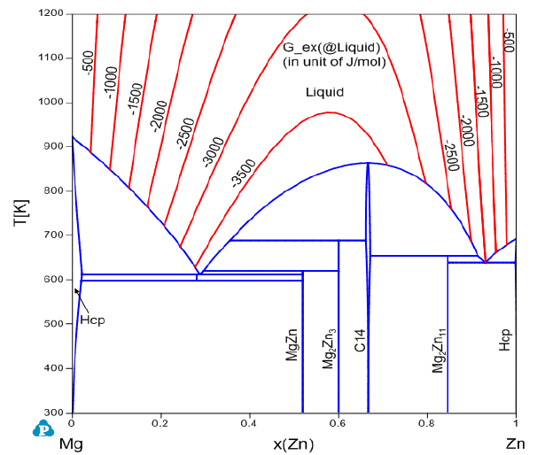
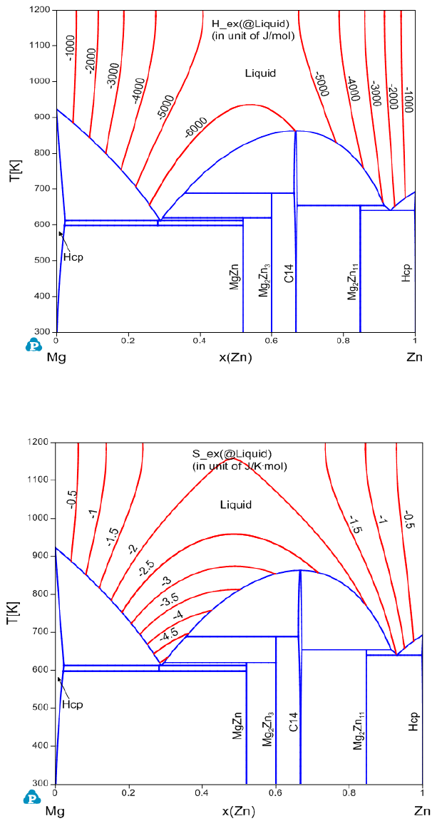
3.3.5.4 Excess Molar Property Diagram
Sometimes we have interest in the excess properties, such as excess Gibbs free
energy, excess enthalpy and excess entropy of a phase. These properties are
available from the property definitions of G_ex, H_ex and S_ex in a contour
diagram. Figure 3.35, Figure 3.36 and Figure 3.37 show the calculated contour
curves for the excess properties of liquid in the Mg-Zn system.
Figure 3.35 Contour diagram of the excess Gibbs free energy in the liquid
phase of Mg-Zn system.
72
Figure 3.36 Contour diagram of the excess enthalpy in the liquid phase of Mg-
Zn system.
Figure 3.37 Contour diagram of the excess entropy in the liquid phase of Mg-
Zn system.
73
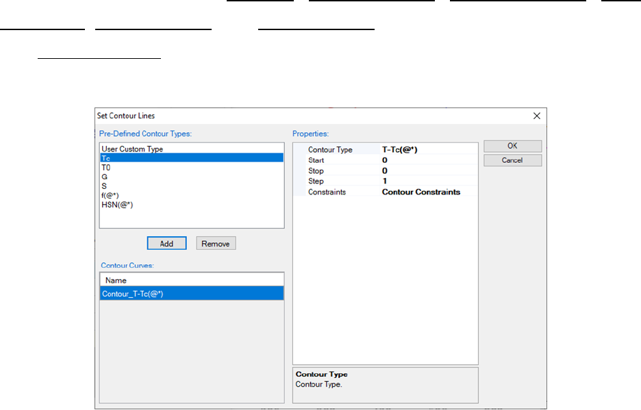
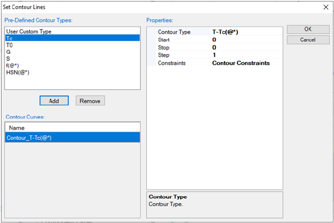
3.3.5.5 User Defined Contour Diagram
Contour diagram can be any type of customized properties defined by the user
using a mathematical expression. Contour diagram can therefore be used to
plot some special property lines. For example, we want to calculate Curie
temperature Tc curves in the Fe-Cr system. A Tc curve can be considered as a
special contour line when T equals to Tc, which means the constraint: T-Tc=0
is set on the Tc curve. Figure 3.38 is the input window for calculating the Tc
contour curves. Since the constraint is T-Tc(@*)=0, the “Start” and “Stop”
values are both set to be zero, and “Step” value is ignored. @* means in every
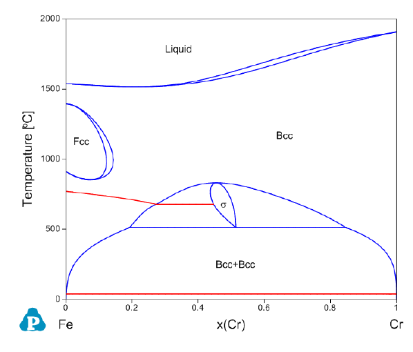
phase. Figure 3.39 is the calculated Fe-Cr phase diagram with the Tc curves of
the Bcc phase.
Figure 3.38 Input windows for Tc curves in Fe-Cr system
74
Figure 3.39 Phase diagram of Fe-Cr with Curie temperature curves (in red
color) of Bcc phase
A second order transition curve could also be calculated as a contour curve.
Fe-Al binary system [2009Sun] is given as an example here. Figure 3.40 is the
calculated Fe-Al binary phase diagram with Tc curves and the second order
transition curves. The Tc curves can be calculated the same way as that shown
in this section for the Fe-Cr system.
The calculation of the second order transition needs special contour property
definition. For the Bcc/B2, the contour property is defined as
abs(y(Fe#2@BCC_4SL)-y(Fe#3@BCC_4SL))
which represents the absolute value of the difference between the site fractions
of Fe on the 2
nd
and 3
rd
sublattices. The “start” and “stop” values are set to
be “0.05”, which avoids the numerical difficulty in calculation and gives a very
good approximation of the order/disorder transition curves.
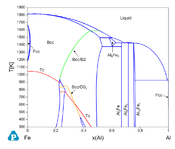
75
Figure 3.40 Phase Diagram of Fe-Al with the Tc curves and the 2
nd
order
transition curves between Bcc and B2 and between B2 and D0
3
.
The contour property for the second order transition between B2 and D0
3
is
defined as
abs(y(Fe#3@BCC_4SL)-y(Fe#4@BCC_4SL))
with the “start” and “stop” values of “0.05”. A constraint is also added in this
contour calculation to make sure that the first and second sublattices have the
same site fractions,
abs(y(Fe#1@BCC_4SL)-y(Fe#2@BCC_4SL))<0.001
Pandat
TM
batch file is written in the language of XML(Extensible Markup
Language). The less-than “<” and great-than “>” characters are reserved as the
XML special characters. In an XML file, the less-than “<” and great-than “>”
symbols are written as “<” and “>”. Above constraint is written in a
Pandat batch file as
abs(y(Fe#1@BCC_4SL)-y(Fe#2@BCC_4SL))<0.001
76
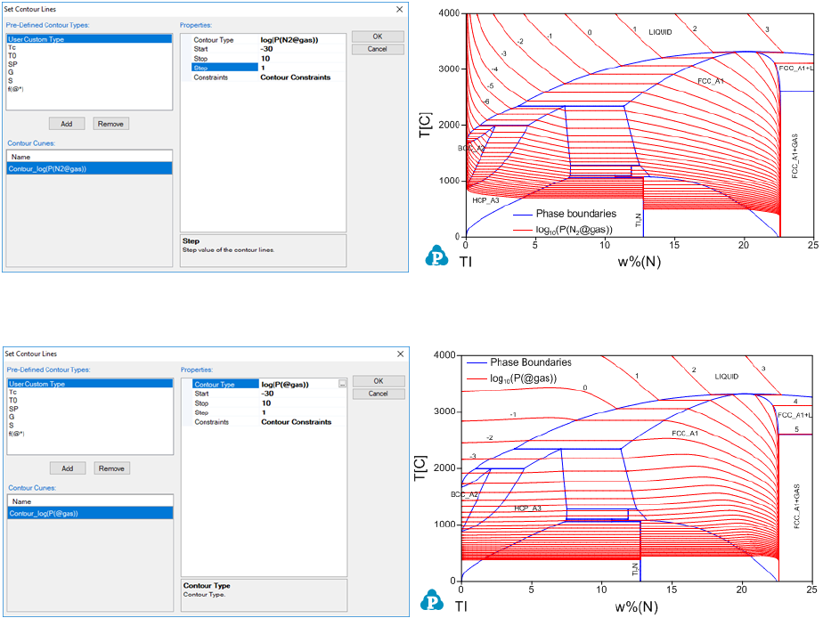
3.3.5.6 Partial Pressure Contour Diagram
The following example shows how to calculate the contour lines for the partial
pressure of the gas phase in the Ti-N system [1996Zen]. Figure 3.41 (a) is the
input condition window and Figure 3.41 (b) is the calculated phase diagram of
Ti-N with the contour lines of log(P(N
2
@gas)) (pressure unit is Pa), which is the
common logarithm of the partial pressure of N
2
in gas. Figure 3.41 (c) is
another input condition window and Figure 3.41 (d) is the calculated phase
diagram of Ti-N with the contour lines of log(P(@gas)), which is the common
logarithm of the total pressure of gas with the gas species N, N
2
, N
3
and Ti.
(a) Input condition (b) log(P(N
2
@gas)) contour
(c) Input condition (d) (log(P(@gas)) contour
Figure 3.41 Contour diagrams of partial pressure of gas in the Ti-N system
More examples can be found in the Pandat example folder:
/PanPhaseDiagram/Contour/.

77
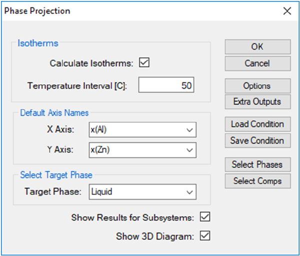
3.3.6 Phase Projection
This function permits the calculation of a phase projection diagram for a
system with two or more components. PanEngine automatically searches the
univariant phase projection lines.
Go to PanPhaseDiagram on the menu bar and select Phase Projection or
Click the button on the tool bar. The Phase Projection dialog box shown in
Figure 3.42 allows the user to calculate projection of any phase in the system.
If “Liquid” is selected as Target Phase, liquidus projection for the system is
calculated. Isothermal curves involving the selected phase in a ternary system
can also be calculated by checking the box Calculate Isotherms. The density
of isothermal curves depends on the scale of Temperature Interval. A larger
value for the temperature interval leads to fewer isothermal curves but with
faster speed of calculation. The default Compositional Range is full range for
each component. User can define the default output graph by selecting the X
and Y axis. User can also access the Options, Extra Outputs, Load Condition,
Save Condition, Select Phases, and Select Comps windows through this
dialog box. If the Show Results for Subsystems box is checked, the output
files will include the results for the subsystems together with the
multicomponent system. Be aware that the output table will be huge if the box
is checked for a calculation with a higher order multi-component system. User
can choose the specific phase for projection calculation in the Target Phase
dialog, such as Fcc phase. If “*” is selected, the projection for all the phases will
be calculated. If the Show 3D Diagram box is checked, there will be an extra
3D diagram showing the calculation results as well as the original 2D diagram.
For the 3D diagram, user can rotate the diagram by holding the left button of
mouse and move it around.
78
Figure 3.42 Phase projection calculation setting dialog
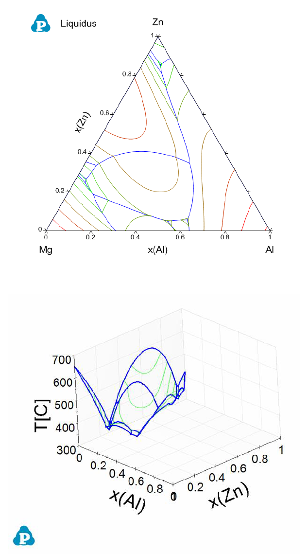
The results from a liquidus projection calculation are displayed in two types of
format in the Pandat
TM
main window: Graph and Table. Figure 3.43 to Figure
3.46 show the 2D and 3D graph view, default table and isotherm table for the
liquidus projection calculation results, respectively. Users can switch between
Graph view to Table View by double clicking on the graph name or the table
name in the Pandat
TM
Workspace window. Extensive operations on Graph and
Table, such as labeling and adding legend, have been discussed in details in
Section 2.3 and Section 2.4.
79
Figure 3.43 Liquidus projection in 2D of the Al-Mg-Zn ternary system
Figure 3.44 Liquidus projection in 3D of the Al-Mg-Zn ternary system
80
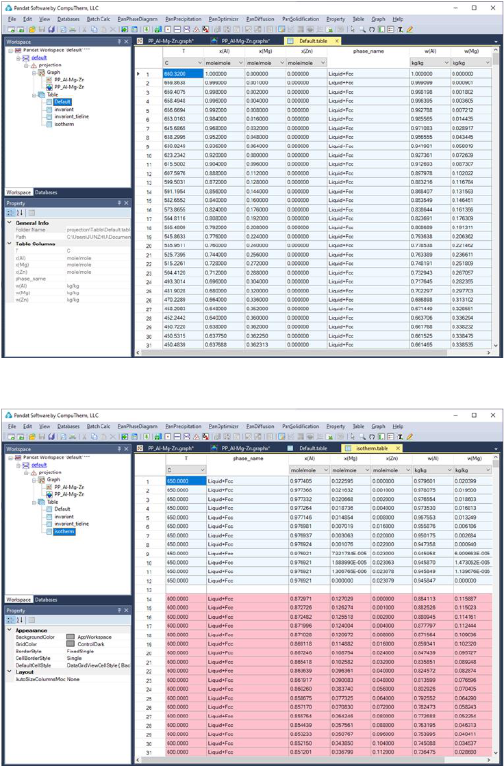
Figure 3.45 Default table view for the liquidus projection calculation results
Figure 3.46 Isotherms table for the liquidus projection calculation results
81
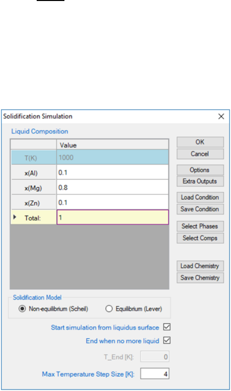
3.3.7 Solidification Simulation
Two simple models, equilibrium solidification and Scheil solidification, have
been integrated into Pandat
TM
for calculating solidification pathways. The
equilibrium model, also called the lever rule model, assumes that complete
diffusion occurs in both liquid and solid phases, and the compositions of solid
and liquid always follow the phase boundaries defined by the equilibrium
phase diagram. The fractions of liquid and solid can be calculated through the
lever rule. In contrast, Scheil solidification assumes that no diffusion occurs in
the solid phases, that the composition of liquid phase is uniform (infinite
diffusivity in liquid) and that local equilibrium at the solid-liquid interface is
always maintained. The Solidification Simulation function calculates the
solidification path of an alloy using either the lever rule or Scheil model as
being decided by the user.
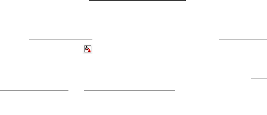
Go to PanPhaseDiagram on the menu bar and select Solidification
Simulation or click the button on the tool bar. The dialog box as shown in
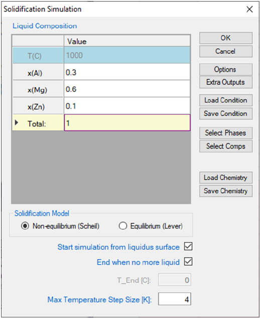
Figure 3.47 allows the user to set up the alloy composition for the solidification
simulation. User can choose the simulation under either Non-
Equilibrium(Scheil) or Equilibrium (Lever Rule) condition. There are two
check boxes at the bottom of the input dialog: Start simulation from liquidus
surface, and End when no more liquid. If both boxes were checked, the
solidification simulation will be carried out in the temperature range when
solid start to form from liquid (liquidus surface) to the point when liquid just
completely disappear. Pandat
TM
software will find these two points
automatically. If one or both of the check boxes are not checked, user will need
to define the start or/and the end temperature for the solidification simulation
proceeds.
82
Figure 3.47 Set calculation conditions for solidification simulation
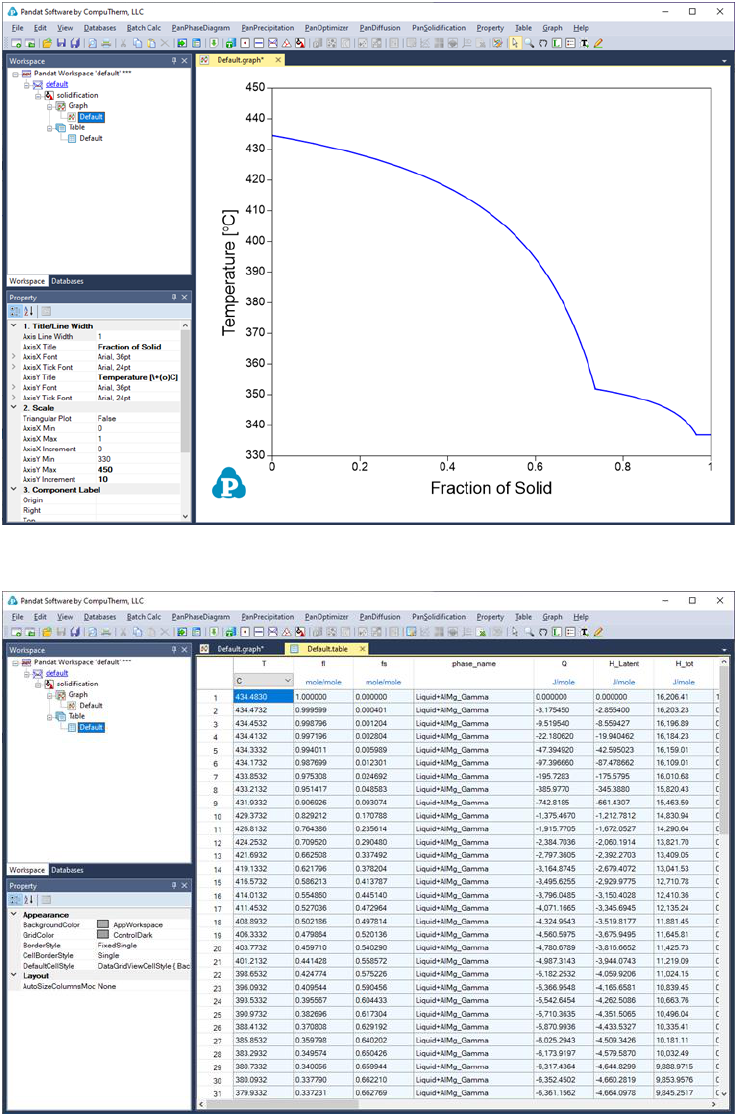
The results are displayed in either Graph View or Table View. Figure 3.48 and
Figure 3.49 show the graph view and table view for the solidification simulation
results with the calculation condition shown in Figure 3.47. Extensive
operations on Graph and Table, such as labeling and adding legend, have been
discussed in details in Section 2.3 and Section 2.4.
PanSolidification, a new module introduced in Pandat 2020, is considered the
back diffusion in the solid phase during solidification. Detailed description on
PanSolidification module is in section 7.
83
Figure 3.48 Graph view of the solidification simulation result
Figure 3.49 Table view of the solidification simulation result
3.3.8 Table Column Functions
Examples are given in this section show how to use the table column property
names and functions to obtain more information from the calculated results.

84
3.3.8.1 Activity and activity coefficient
The activity of a component j,
, is defined by
where
is the chemical potential of the component j in equilibrium state and
is the chemical potential of this component at its reference state. For
example, the activity of component Al in the liquid Al-Mg system referring the
Al in Fcc phase is calculated by
The corresponding Table column name is a(Al@Liquid:Fcc[Al]), or
a(Al@Liquid:Fcc).
If a reference state is not specified in Table column name, the default reference
state in the database is taken as the reference state. For example,
a(Al@Liquid) is calculated by
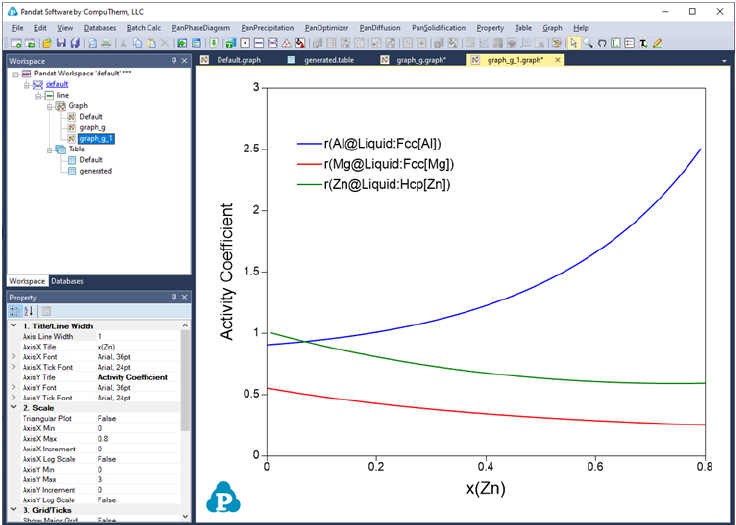
Activity coefficient is defined as
which is available from Table by defining Table column name similar to that of
activity. Table column name for the activity coefficient of Al in liquid is
r(Al@Liquid:Fcc[Al]), or r(Al@Liquid:Fcc).
Figure 3.50 to Figure 3.53 show the screen images for creating a table of
activity and activity coefficient from a line calculation result at 1000K in the Al-
Mg-Zn ternary system. The two end points are at x(Mg)=0.2,x(Al)=0.8 and
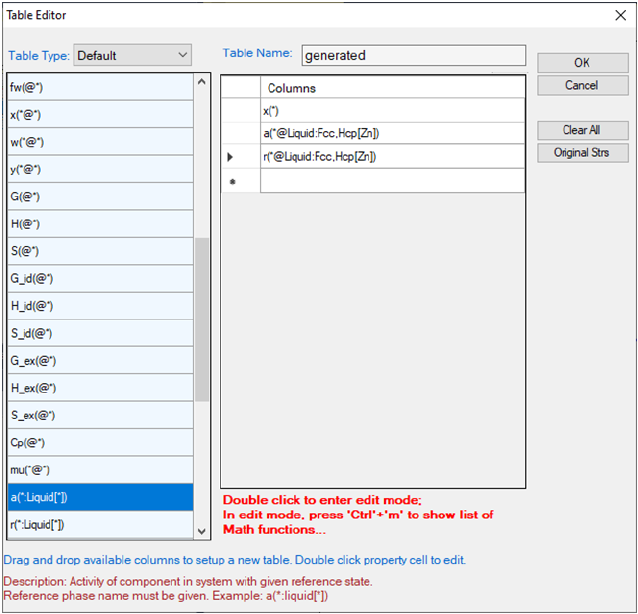
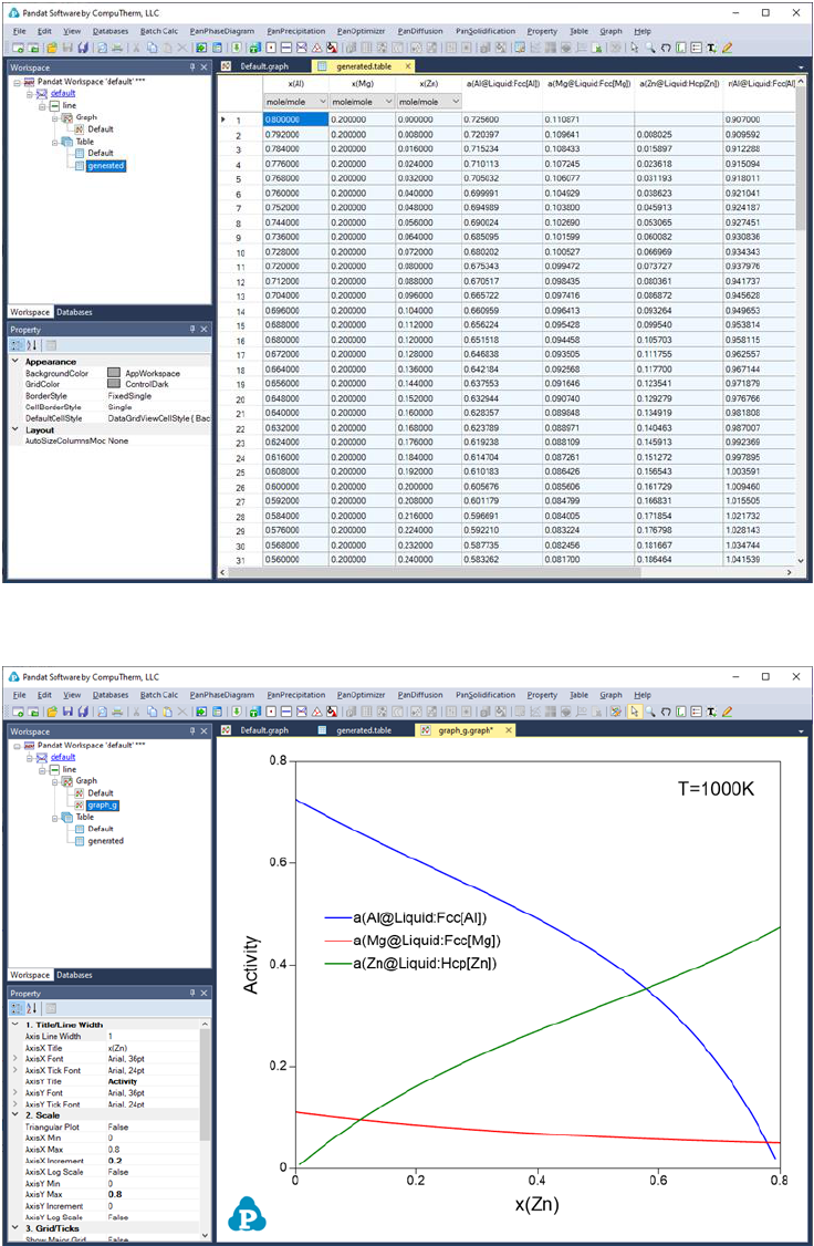
86
Figure 3.51 Table of activity and activity coefficient
Figure 3.52 Graph of activity vs. x(Zn)
88
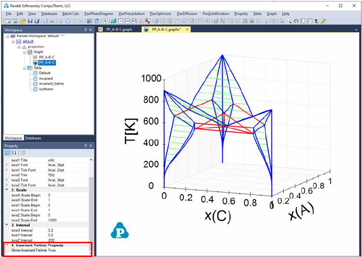
Figure 3.54 is a 3D ternary phase diagram calculated from the database file
“ABC.tdb” which is provided in the Pandat Examples. This system has three
binary eutectic reactions. To show the invariant tielines in these binaries, set
the “Show Invariant Tieline” in the Property window as “true”, then the
invariant lines will be plotted on it as shown in Figure 3.55.
Figure 3.54 3D phase projection of a simple ternary system with eutectic
reaction in every binary system
89
Figure 3.55 3D phase projection with three binary eutectic and one ternary
eutectic tielines shown as red
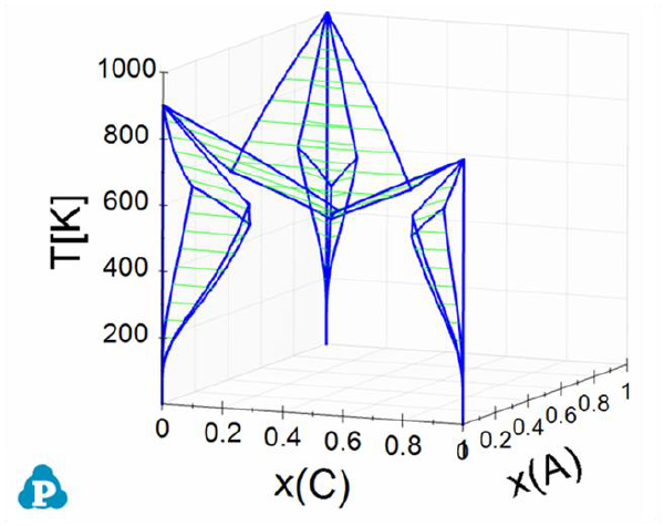
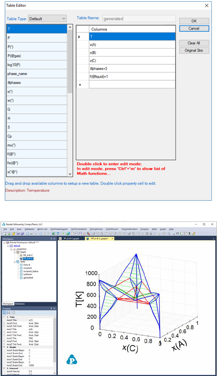
The ternary univariant lines (L+Bcc+Fcc, L+Bcc+Hcp, and L+Fcc+Hcp, magenta
color) connects these reactions can be highlighted as follows. First, create a
new table as shown in Figure 3.56. The purpose of the new table is to extract
the boundary line(s) that connect Liquid, and the other two solid phases, and
the fraction of Liquid on this boundary line is 1. After the table is created,
select this new table in the Explore window, and drag x(C) from the Property
window to the Main Display window, and drop it as the x-axis; press “Ctrl” and
then drag x(A) from the Property window to the Main Display window, and drop
it as the y-axis; press “Shift” and then drag T from the Property window to the
Main Display window, and drop it as the z-axis. This line showing the gradually
change from the peritectic reaction to the eutectic reaction is then highlighted
(green color), as shown in Figure 3.57.
90
Figure 3.56 Create a new table to extract the ternary univariant lines
91
Figure 3.57 The ternary univariant lines (green lines) connecting the two
invariant reactions in the two binaries
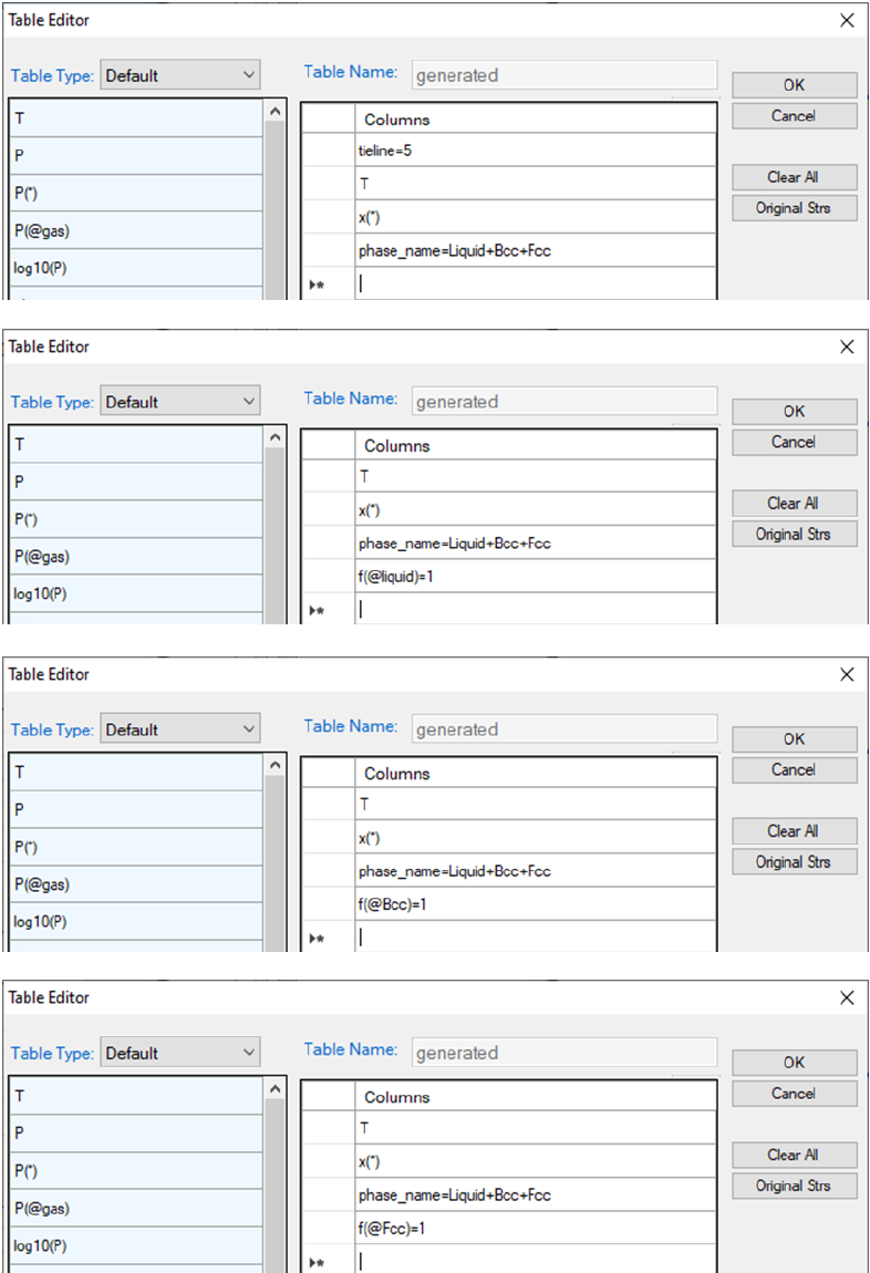
Figure 3.58 shows how to create 4 new tables to plot the 3D diagram in Figure
3.59, which shows the ternary three-phase equilibrium tie-triangle volume. The
4 tables include a set of the tie-triangles by setting its density as "tieline=5"
and the phase lines for the liquid, Bcc, Fcc phases by setting the fraction of the
corresponding phase to be 1.
92
Figure 3.58 Create tables to extract tie-triangles and the three edges of the
three-phase volume.
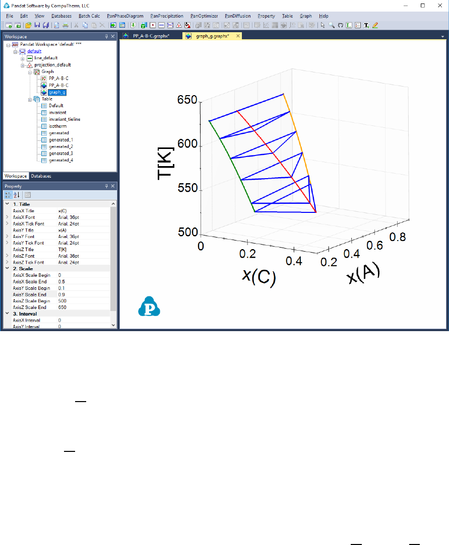
93
Figure 3.59 3D diagram of the three-phase volume.
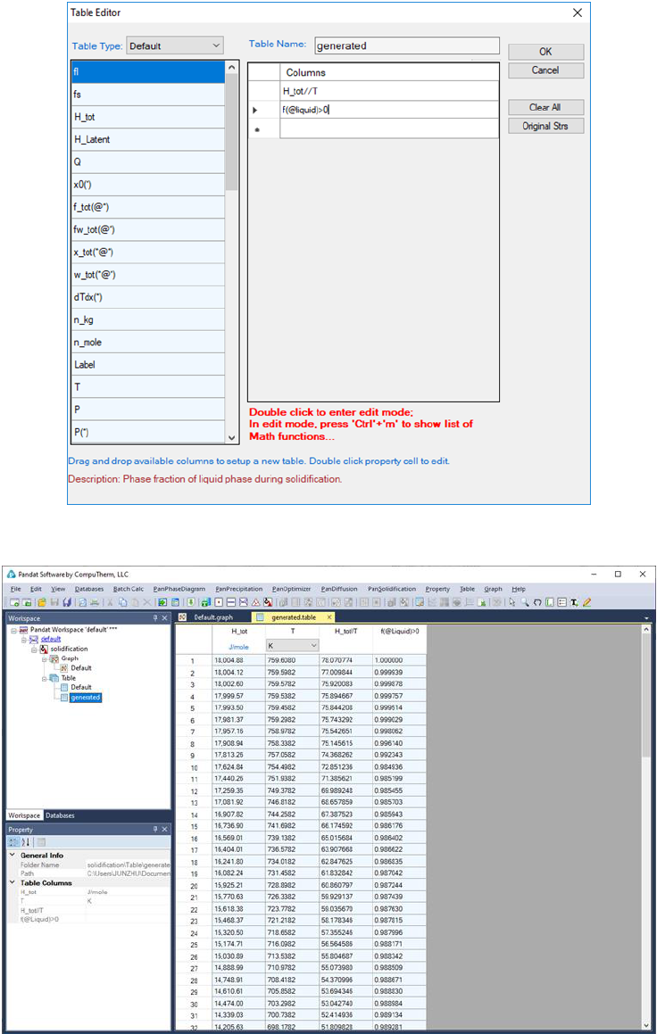
3.3.8.3 Numerical derivative
The derivative
can be calculated numerically from the two columns of Y and
Z. The operator for numerical derivative is “//”, double slashes. The numerical
derivative of
is written in the form of “Y//Z” as the column name. Only one
numerical derivative operator is allowed in one column. In other words, user
cannot type in “Y//Z//X”.The derivative “Y//Z” will be parsed into three
columns in the new table: “Y”, “Z” and “Y//Z”, which makes it easy for the user
to view the original data set “Y”, “Z” and choose to plot either
vs Z or
vs Y.
The example given here is to find the “effective heat capacity” of the system
during solidification (H_tot//T). A system of Al-Mg-Zn is chosen and the
composition is shown in Figure 3.60. After Scheil simulation is done, a new
table is created with the definition of the column names shown in Figure 3.61.
94
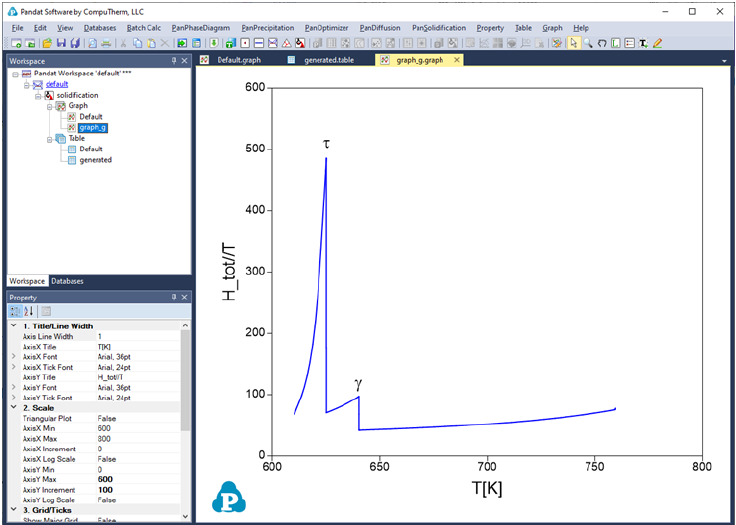
Figure 3.62 is the newly generated table. Select the columns “T” and
“H_tot//T”, we have the
vs T diagram as in Figure 3.63. This diagram
shows the effective heat capacity change during the solidification by Scheil
simulation. There are two peaks in Figure 3.63, which represent roughly the
phase transformation from liquid to Hcp+γ and that from liquid to Hcp+,
respectively.
Figure 3.60 Solidification simulation condition.
95
Figure 3.61 Create a table for the numerical derivative of H_tot w.r.t. T.
Figure 3.62 The table for the numerical derivative of H_tot w.r.t. T.
96
Figure 3.63 plot of effective heat capacity change during the solidification
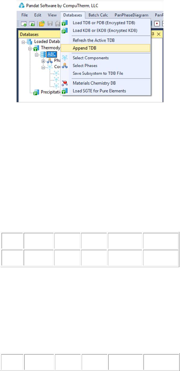
3.3.9 Append Database
On top of the original database (*.tdb or *.pdb) loaded from Pandat GUI, user
can append a custom-made database (*.tdb) by select the Append TDB
function from the Databases menu as shown in Figure 3.64.
Using this function, user can (1) replace the value of an existing parameter, (2)
add value to an existing parameter, (3) add new parameters to an existing
phase, (4) add new phases to the original database, and (5) add user-defined
properties. In the following, the hypothetical A-B system will be used as
example to explain the Append TDB function in detail.
97
Figure 3.64 Append TDB function under the Databases menu
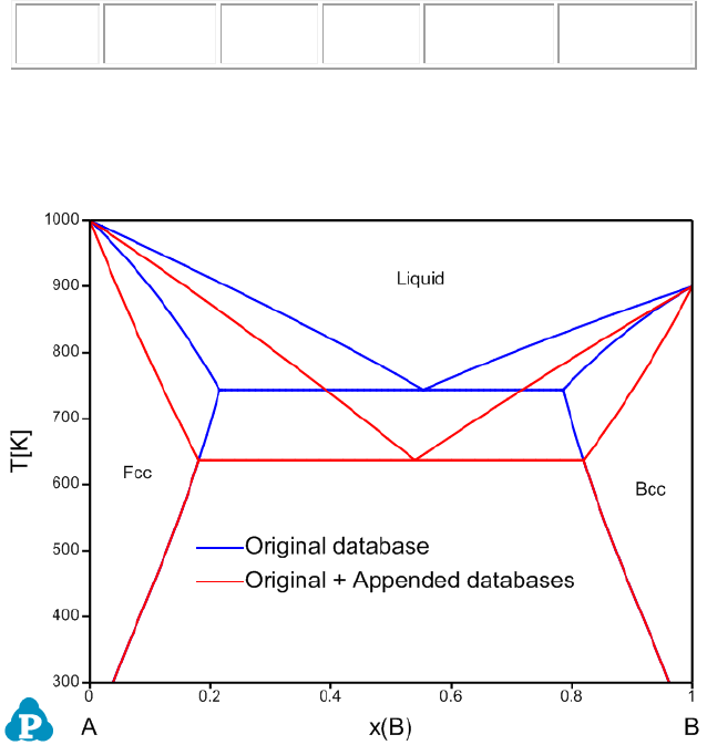
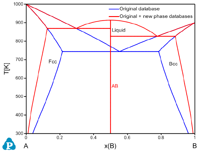
3.3.9.1 Replace the Value of an Existing Parameter
In this example, we are going to replace the interaction parameter of the liquid
phase: G(Liquid,A,B;0) within the original AB_original.tdb database. Load the
AB_original.tdb from the Databases menu by selecting the Load TDB or PDB
function. The interaction parameter of G(Liquid,A,B;0) described in the original
database is expressed as:
Parameter G(Liquid,A,B;0) 298 3000; 6000 N !
In the TDB Viewer, one can see the original value of G(Liquid,A,B;0)=3000.
Name
Property
x-Term
x-order
Parameter
T-limit (K)
L
(A,B)
0
3000
6000
In the AB_replace parameter.tdb, only the interaction parameter for
G(Liquid,A,B;0) is defined, but with a different value:
Parameter G(Liquid,A,B;0) 298 -2000; 6000 N !
Load the AB_replace parameter.tdb via the Append TDB function, one can see
from the TDB Viewer that the interaction parameter of G(Liquid,A,B;0) is
replaced with the value (-2000) from the appended database.
Name
Property
x-Term
x-order
Parameter
T-limit (K)
98
Liquid
L
(A,B)
0
-2000
6000
The calculated phase diagrams using both original database and original +
appended databases are shown in Figure 3.65.
Figure 3.65 Calculated A-B phase diagram using both original database and
original + appended databases
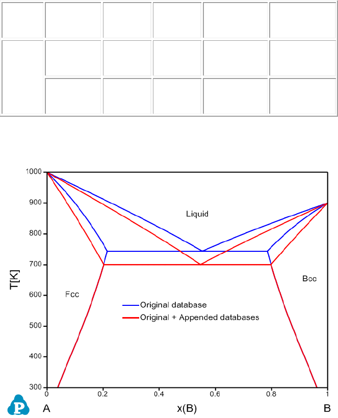
3.3.9.2 Add Value to an Existing Parameter
In this example, we are going to modify the interaction parameter of the liquid
phase G(Liquid,A,B;0) within the original AB_original.tdb database by adding a
value to it. As shown in the AB_modify parameter.tdb, the interaction
parameter is expressed as GG(Liquid,A,B;0), which means adding this
assigned value to the original value rather than replacing it.
Parameter GG(Liquid,A,B;0) 298 -2000; 6000 N !
As shown in the above section 3.3.9.1, the original value of the G(Liquid,A,B;0)
interaction parameter is +3000. When we append the AB_modify parameter.tdb
to the original database, the value of -2000 will be added to the original value
+3000 for the G(Liquid,A,B;0) interaction parameter. As shown in the TDB
viewer below, one extra term “GG” is listed. For this case, the total value of the
99
interaction parameter of G(Liquid,A,B;0) will be modified to be 3000 + (-2000) =
+1000.
Name
Property
x-Term
x-order
Parameter
T-limit (K)
Liquid
L
(A,B)
0
3000
6000
GG
(A,B)
0
-2000
6000
The calculated phase diagrams using both original database and original +
appended databases are shown in Figure 3.66.
Figure 3.66 Calculated A-B phase diagram using both original database and
original + appended databases with adjusted parameters
Note that, the Append TDB function allows user to append only one database
to the original database. When user wants to append another database to the
original database, the previously appended database will need to be removed
first. Pandat
TM
will notify the user as shown in Figure 3.67 and user need to
click Yes to confirm.
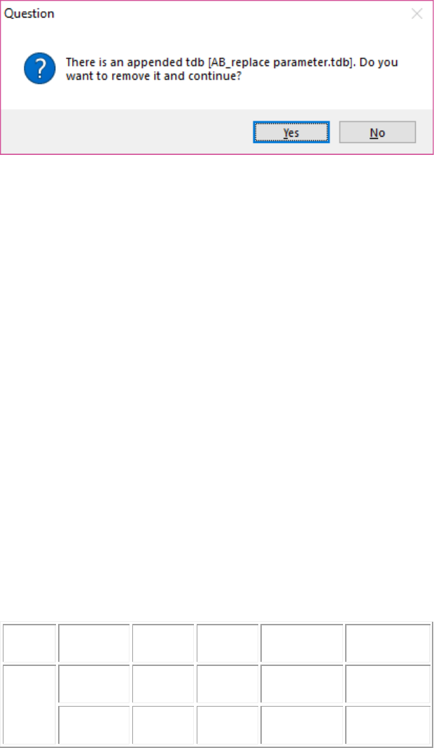
100
Figure 3.67 Append database confirmation
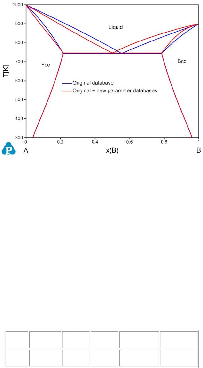
3.3.9.3 Add New Parameter to an Existing Phase
In addition to replace or modify the existing parameters for an existing phase in
the original database, one can also add new parameters to this phase. In the
AB_Original.tdb database, there is only one interaction parameter for the
Liquid phase G(Liquid,A,B;0). Using the Append TDB function, we can add
more interaction parameters to the Liquid phase. As shown in the AB_new
parameter.tdb, another interaction parameter for the liquid phase,
G(Liquid,A,B;1), is given as:
Parameter G(Liquid,A,B;1) 298 -2000; 6000 N !
Load the original AB_original.tdb and then load the AB_new parameter.tdb via
the Append TDB function. As shown in the TDB viewer, the new interaction
parameter (x-order value is 1) is added.
Name
Property
x-Term
x-order
Parameter
T-limit (K)
Liquid
L
(A,B)
0
3000
6000
L
(A,B)
1
-2000
6000
The calculated phase diagrams using both original database and original +
appended databases are shown in Figure 3.68.
101
Figure 3.68 Calculated A-B phase diagram using both original database and
original + appended databases with new parameters
3.3.9.4 Add New Phases to the Original Database
In addition to modify the parameters for existing phases within the original
database, one can also add new phases via the Append TDB function. A new
phase AB is introduced in the AB_new phase.tdb, which is described as:
Phase AB % 2 0.5 0.5 !
Constituent AB :A:B:!
Parameter G(AB,A:B;0) 298.15 -10000+6*T; 6000 N !
Load the AB_original.tdb first and then load the AB_new phase.tdb via the
Append TDB function. As shown in the TDB Viewer, a new AB phase is
introduced.
Name
Property
x-Term
x-order
Parameter
T-limit (K)
AB
L0
(A)(B)
0
-10000+6*T
6000
The calculated phase diagrams using both original database and original +
appended databases are shown in Figure 3.69.
102
Figure 3.69 Calculated A-B phase diagram using both original database and
original + appended databases with new phase
3.3.9.5 Add User-defined Properties to the Original Database
As is well known, the CALPHAD method has now been used to describe various
types of phase properties in addition to thermodynamic properties. Mobility
databases, molar volume databases and other thermo-physical property
databases can be developed via similar route as that of developing a
thermodynamic database. The Append TDB function allows a user to add
user-defined properties to an original database. In this example, we add molar
volume to AB_Original.tdb via the Append TDB function. The molar volume
parameters of A and B within the Bcc, Fcc, and Liquid phases are described in
the AB_property.tdb database as listed below:
Parameter Vm(Bcc,A;0) 298.15 +7.4e-6*exp(1e-6*T); 3000 N !
Parameter Vm(Bcc,B;0) 298.15 +8.4e-6*exp(1e-6*T); 3000 N !
Parameter Vm(Fcc,A;0) 298.15 +7.0e-6*exp(1e-6*T); 3000 N !
Parameter Vm(Fcc,B;0) 298.15 +8.0e-6*exp(1e-6*T); 3000 N !
Parameter Vm(Liquid,A;0) 298.15 +8.0e-6*exp(1e-6*T); 3000 N !
103
Parameter Vm(Liquid,B;0) 298.15 +9.0e-6*exp(1e-6*T); 3000 N !
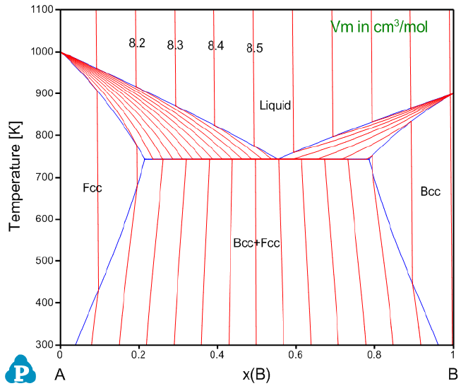
Load the original database AB_original.tdb and then append the
AB_property.tdb database via the Append TDB function. The currently
combined AB_original + AB_property database enables us to calculate molar
volume of the A-B binary system in addition to the phase diagram. The molar
volume contour lines are shown in Figure 3.70 (refer to Section 3.3.5 for
calculating contour diagrams). Moreover, density and linear thermal expansion
coefficient can also be calculated with this AB_original + AB_property database.
Please note that, various types of user-defined properties including but not
limited to atomic mobility, molar volume, viscosity, surface tension can all be
combined with the original thermodynamic database via the Append TDB
function.
Figure 3.70 Calculated A-B phase diagram using both original database and
original + appended databases with specific property
104
3.3.10 User-defined Property
This section is an extension of the above Append database section to develop
and add user-defined-property database to the original database. Pandat allows
user to define any property of a phase in a format similar to that of the Gibbs
energy describing a disordered solution phase. Let U be the user-defined
property and it is expressed as:
1
1 1 1
()
c c c
o k k
i i i j i j ij
i i j i k
U xU x x x x L
−
= = = +
= + −
where
i
x
is the molar fraction of component i and
0
i
U
is the property of the pure
component i,
k
ij
L
is the k
th
order interaction parameter between components i
and j.
User can also define special properties associated with the properties of phases
in the original database. Any phase property available from Pandat Table can
be used for user-defined property, such as G, H, mu, and ThF. However, the
star symbol in a property, like mu(*), cannot be used. User may refer to
section 8 for more properties in detail.
3.3.11 Advanced Features
In this section, we are going to cover some advanced features of the
PanPhaseDiagram module.
3.3.11.1 Local Equilibrium
In default, Pandat always calculates global stable phase equilibria. Even some
phases are suspended, the calculated phase equilibria are still global stable
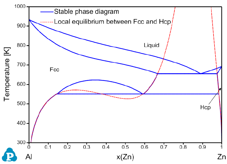
ones for those “Entered” phases. The current version of Pandat enables us to
calculate a “real” local equilibrium. The Al-Zn binary system is used as an
example to demonstrate how to calculate the local phase equilibrium between
the Fcc and Hcp phases. Note that, there is not GUI for the local equilibrium
function and user has to run it through the batch file (.pbfx).
105
As shown below, a point with initial values needs to be defined in the batch file.
<point>
<statespace>
T value="500"/>
<P value="1"/>
<n component="Al" value="0.5"/>
<n component="Zn" value="0.5"/>
</statespace>
<initial_value>
<mu species="Al" value="-16000" />
<mu species="Zn" value="-22000" />
<phase_point phase_name="Fcc">
<y species="Al" sublattice="1" value="0.9" />
<y species="Zn" sublattice="1" value="0.1" />
</phase_point>
<phase_point phase_name="Hcp">
<y species="Al" sublattice="1" value="0.01" />
<y species="Zn" sublattice="1" value="0.99" />
</phase_point>
</initial_value>
</point>
In addition to the point with initial values, equilibrium type needs to be set as
“local” (as shown below)
<condition>
<equilibrium_type type="local"/>
106
</condition>
Figure 3.71 is the calculated stable Al-Zn binary phase diagram with the local-
equilibrium between Fcc and Hcp phases.
Figure 3.71 Calculated Al-Zn stable phase diagram with local-equilibrium
between Fcc and Hcp phases
3.3.11.2 Hessian matrix of Gibbs energy
Pandat can calculate the determinant of Hessian matrix of Gibbs energy of a
phase and the eigenvalues and eigenvectors of the Hessian matrix.
Since there is one dependent molar fraction for the molar fraction
variables
, one of the components is selected as the dependent one.
Without loss of generality,
is selected as the one, i.e., the last component is
considered as the solvent. Then, the second derivatives of Gibbs free energy of
a phase form the Hessian matrix, which is an
symmetrical
matrix.

107
Its determinant is given by
The determinant of Hessian matrix for phase f is available from “HSN(@f)”. The
value of “HSN(@f)” is independent of the selection of solvent component.
A Hessian matrix has real eigenvectors and each eigenvalue has a
corresponding eigenvector. The eigenvalues and their eigenvectors are available
from “eVal(#*@f)” and “HSN(*#*@f)”. Above Hessian matrix has eigenvalues
of “eVal(#1@f)”, eVal(#2@f)”, ,“eVal(#n-1@f)”. Each eigenvalue has an
eigenvector. For example, eVal(#1@f) has a eigenvector of (eVec(C
1
#1@f),
eVec(C
2
#1@f), , eVec(C
n-1
#1@f)), where C
k
is the name of the k
th
component.
108
Table 3.1 Functions that can be used in database and Table operation
Function
Meaning
sin(x), cos(x), tan(x),
tan2(y,x)
Trigonometric functions. tan2(y,x)=tan(y/x)
asin(x), acos(x),
atan(x), atan2(y,x)
Arcus functions. atan2(y,x)= atan(y/x)
sinh(x), cosh(x),
tanh(x)
Hyperbolic functions
asinh(x), acosh(x),
atanh(x)
Arcus hyperbolic functions
Log2(x), log10(x), ln(x)
Logarithm functions to base 2, 10 or e
exp(x)
exponential function
abs(x)
absolute value
sqrt(x)
square root
rint(x)
round to integral value
sign(x)
sign function
HSN(@*)
determinant of Hessian matrix of Gibbs free energy of a
phase
eVal(#*@*)
eigenvalues of Hessian matrix of Gibbs free energy of a
phase. * after # represents the eigenvalue index
eVec(*#*@*)
eigenvectors for the eigenvalues of Hessian matrix of Gibbs
free energy of a phase. * before # represents the component
of eigenvector. * after # represents the eigenvalue index.
The “solvent” component can be defined while using “Thermodynamic Property”
calculation, or defined in Pandat Batch file. If “solvent” component is not
defined, Pandat will choose the first component (the smallest atomic number)
as the default “solvent” component.