123
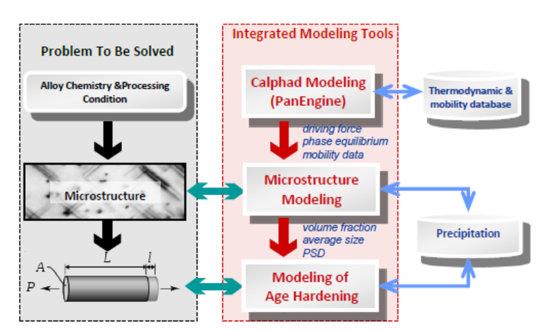
5 PanPrecipitation
A module of Pandat
TM
software, which is seamlessly integrated with the
thermodynamic calculation engine – PanEngine for the necessary
thermodynamic input and mobility data, is designed for the simulation of
precipitation kinetics during heat treatment process. It is built as a shared
library and integrated into Pandat as a specific module that extends the
capability of Pandat for kinetic simulations, while taking full advantage of the
automatic thermodynamic calculation engine (PanEngine) and the user-friendly
Pandat Graphical User Interface (PanGUI). For this reason, precipitation
simulations for highly complex alloys under arbitrary heat treatment
conditions can be accomplished with only a few operations. Error! Reference
source not found. shows the three-layered architecture of this modeling tool.
Figure 5.1 The three-layered architecture of the integrated modeling tool
5.1 Features of PanPrecipitation
5.1.1 Overall Design
➢ Concurrent nucleation, growth/dissolution, and coarsening of precipitates
124
➢ Temporal evolution of average particle size and number density
➢ Temporal evolution of particle size distribution
➢ Temporal evolution of volume fraction and composition of precipitates
5.1.2 Data Structure
PanPrecipitation is a purely object-oriented module written in C++ with generic
data structures like PanEngine, balancing performance, maintainability and
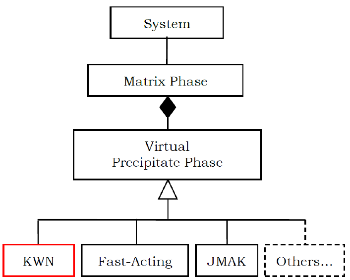
scalability. The basic data structure for storing precipitation information in the
system of interest is schematically shown in Figure 5.2.
Figure 5.2 Data structure of system information in PanPrecipitation
In general, a system contains a matrix phase and a number of precipitate
phases. Different precipitate phases may behave differently, which should be
described by different kinetic models. On the other hand, the calculation speed
is directly related to the complexity of the model. It therefore requires multi-
level models for different purposes. The current PanPrecipitation module
includes two built-in models: the Kampmann/Wagner Numerical (KWN) model
and the Fast-Acting model. One unique advantage is that this generic data
125
structure allows easy integration of other precipitation models with the
PanPrecipitation module as shown in Figure 5.2. This gives users great
flexibility in choosing the proper kinetic models, including their own user-
defined models, for custom applications.
Based on the above data structure, input parameters for the matrix and its
precipitate phases are organized in “Extensible Markup Language” (XML)
format, which is a standard markup language and well-known for its
extendibility. In accordance with the XML syntax, a set of well-formed tags are
specially designed to define the kinetic model for each precipitate phase and its
corresponding model parameters such as interfacial energy, molar volume,
nucleation type, and morphology type. In PanPrecipitation, two kinetic models
known as the KWN and Fast-Acting were implemented and available for user’s
choice. Both models can be used to simulate the co-precipitation of phases
with various morphologies (sphere and lens), with concurrent processes of
nucleation, growth and coarsening. With the selection of the KWN model, the
particle size distributions (PSD) of various precipitate phases can be obtained
in addition to the temporal evolution of the average size and volume fraction as
obtained from the Fast-Acting model. Therefore, the KWN model is
recommended by default.
5.1.3 Kinetic Models
In PanPrecipitation, KWN model is based on the Kampmann and Wagner’s
work as implemented in a numerical framework, and extended to handle both
homogeneous and heterogeneous nucleation, dealing with various
morphologies for the simulation of precipitation kinetics of multi-component
alloys under arbitrary heat treatment conditions. The following is a brief
introduction to the KWN model along with its sub-models for nucleation,
growth and coarsening.
Specifically, in the KWN model the continuous PSD is divided into a large
number of size classes. The program takes a simulation step at every sample

126
time hit. To maintain both accuracy and efficiency between two adjacent
simulation steps, a fifth-order Runge-Kutta scheme is used to generate an
adaptive step size based on the continuity equation.
Please note that all the variables used in the equations in this section are
summarized in Tables 5.1-5.4. Please refer to Tables 5.2-5.4 and examples in
Section 5.1.4 for setting up these variables in the KDB files.
5.1.3.1 Nucleation
(a) Homogeneous nucleation
At each simulation step, the number of new particles is first calculated using
classical nucleation theory and then these new particles are allocated to an
appropriate size class. The transient nucleation rate is given by,
(5.1)
The pre-exponential terms in equation (5.1) are:
, the nucleation site density,
, the Zeldovich factor and
, the atomic attachment rate.
is the time,
the
incubation time for nucleation,
the Boltzmann constant and
T
the
temperature.
The nucleation barrier is defined as
where
*
R
is the radius of
the critical nucleus and
. The nucleation barrier can be written as,
(5.2)
V
G
is the chemical driving force per volume for nucleation and calculated
directly from thermodynamic database with
,
is the elastic strain
energy per volume of precipitate.
is the interfacial energy of the
matrix/particle interface. For a spherical nucleus,

127
(5.3)
(5.4
(5.5
Where
V
is the molar volume of the matrix, and
a
is the lattice constant of the
precipitate phase and
eff
D
is the effective diffusivity
and is
defined by [2004Svo], where
pi
C
is the mean concentration in the precipitate
and
0i
C
is the mean concentration in the matrix phase.
0i
D
is the matrix
diffusion coefficient of the component i.
The calculation of the elastic strain energy is given by Nabarro [1940Nab] for a
homogeneous inclusion in an isotropic matrix,
(5.6)
Where is the shear modulus of the matrix. Thus the elastic strain energy is
proportional to the square of the volume misfit
. The function
provided
in [1940Nab] is a factor that takes into account the shape effects. For a given
volume, a sphere (
) has the highest strain energy while a thin plate (
) has a very low strain energy, and a needle shape (
) lies between the
two. Therefore the equilibrium shape of precipitates will be reached by
balancing the opposing effects of interfacial energy and strain energy. When
is small, interfacial energy effect should dominate and the precipitates should
be roughly spherical.
In homogeneous nucleation, the number of potential nucleation sites can be
estimated by,
(5.7)

128
Where
is the Avogadro number. The value of nucleation site parameter
is
an adjustable parameter and usually chosen close to solute concentration for
homogeneous nucleation.
(b) Heterogeneous nucleation
For heterogeneous nucleation on dislocations, grain boundaries (2-grain
junctions), grain edges (3-grain junctions) and grain corners (4-grain
junctions), the potential nucleation sites
and the nucleation barrier
must be adjusted accordingly.
There are two ways to account for heterogeneous nucleation in
PanPrecipitation. One way is to treat nucleation site parameter
in equation
(5.7) as phenomenological parameters and replace equation (5.2) by a user-
defined equation. An example is given at section 5.1.4.4. The other way is to
theoretically estimate the potential nucleation sites and calculate the
nucleation barrier by assuming an effective interfacial energy for each
nucleation site. For nucleation on grain boundaries, edges or corners, the
nucleation barrier can be calculated by [55Cle],
(5.8)
Where
is the interfacial energy and
is the grain boundary energy and ,
, are geometrical parameters, which are evaluated for grain boundaries,
edges and corners. By introducing a contact angle, the grain boundary energy
can be calculated from
. An effective interfacial energy
is
then introduced and the nucleation barrier is given as
with
(5.9)

129
The effective interfacial energy
can be applied in the framework of classical
nucleation theory. One can verify that the homogenous nucleation equations
are recovered with
.
The potential nucleation sites on grain boundaries can be estimated from the
densities for grain boundary area, grain edge and grain corner, which depend
on the shape and size of grain in the matrix phase,
(5.10)
and
(5.11)
where
are nucleation densities, for bulk nucleation, for grain
boundary nucleation, for grain edge or dislocation nucleation and for
grain corner nucleation. The nucleation densities for grain boundary, edge or
corner are dependent on the grain size and the aspect ratio in
tetrakaidecahedron shape,
(5.12)
where
is a function of and can be estimated for each case.
For nucleation on dislocations, the potential nucleation sites can be calculated
from equation (5.11) if a dislocation density
is given.
(c) Estimation of interfacial energy
The interphase boundary energy between the matrix and a precipitate phase or
interfacial energy is the most critical kinetic parameter in the precipitation
simulation. The generalized broken bond (GBB) method is used to estimate the
interfacial energy for different alloys and temperatures,
(5.13)

130
The prefixed structure factor of 0.329 reflects the average proportion of broken
bonds due to precipitations for fcc and bcc matrix.
is the solution enthalpy
and calculated from thermodynamic database.
is a correction factor for the
size of the precipitate particle.
is a correction factor for diffuse interfaces. It
is a function of
with
being the highest or critical temperature at which two
phases are present in the system. At
, the composition of matrix and
precipitate phases is the same and the interface energy equals to zero. At
, an ideal sharp interface is present.
can be provided by the user in the
kdb file. If
is unknown and not provided,
=1. Such an example is given
in section 5.1.4.2.
131
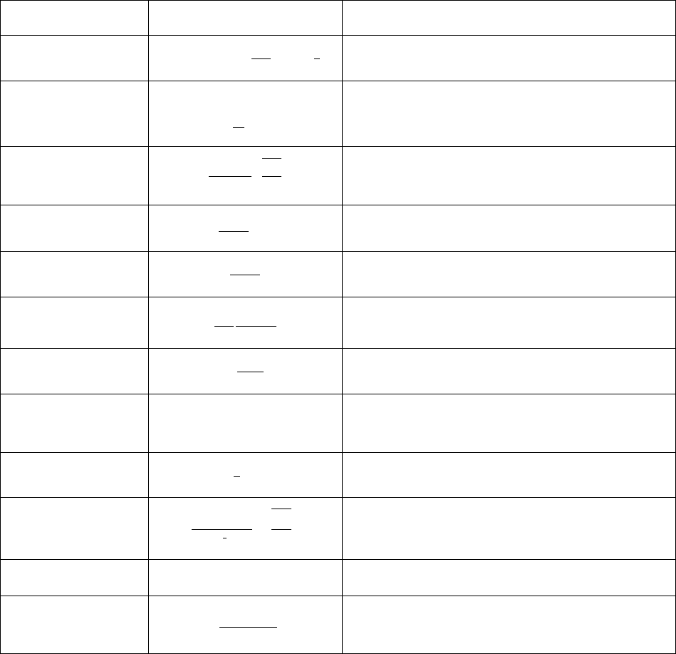
Table 5.1 Summary of equations for nucleation models
Symbol
Equation
Description
The transient nucleation rate
and
Potential nucleation sites
Zeldovich factor
Atomic attachment rate
Incubation time
Nucleation barrier energy
Critical nucleation radius
Volume energy change during nucleation.
is the
chemical driving force per volume and
is the elastic
strain energy
Elastic strain energy. The volume misfit and particle
aspect ratio
are given in kdb file
Effective interfacial energy
The estimated interfacial energy based on GBB method
Effective diffusivity for multi-component alloys

132
5.1.3.2 Growth
Two kinds of growth models are implemented in current PanPrecipitation
module:
(a) Simplified Growth model
The growth of existing particles for each size class is computed by assuming
diffusion-controlled growth, where the Gibbs-Thomson size effect is also taken
into account. The growth model for multi-component alloys proposed by Morral
and Purdy [1994Mor] is adopted in PanPrecipitation and modified to handle the
growth/dissolution of various precipitate phases with different morphologies.
The motion rate of the curved interface, e.g., the interface of a spherical or
lens-like precipitate is given by,
*
22
mm
VV
dR K
v
dt R R R
= = −
(5.14)
where
R
is the radius of the interface.
*
R
is the radius of the critical nucleus
and
(
)
1
1
K
C M C
−
=
.
(
C
and
)
C
are the row and column vector
of the solute concentration difference between
(matrix phase) and
(precipitate phase), and
M
is the chemical mobility matrix. One can verify
that the equation (5.14) can be further simplified and written as,
*
m
dR K
vG
dt R
= =
(5.15)
where
K
is the kinetic parameter, and
*
m
G
is the transformation driving force
defined as
*
m m T
G G G = −
with
m
G
being the molar chemical driving force and
2
m
T
V
G
R
=
compensating the energy difference due to the Gibbs-Thompson
effect.

133
(b) SFFK (Svoboda-Fischer-F-Kozeschnik) Model
The SFFK model [2004Svo] presents a set of linear equations describing the
rate of change of radius and chemical composition of each precipitate in the
system. Let the system consist of a matrix and a number of precipitates. The
composition of each precipitate phase is not without boundary, it is determined
by the complex lattice structure of the precipitate and the thermodynamic
model used to describe the phase. The constraints can be written as,
1
,( 1,..., )
n
ij i j
i
a C U j p
=
==
(5.16)
where the parameters
ij
a
take on the values 0 or 1.
For the description of the state of a closed system under constant temperature
and pressure, the state parameters
i
q
can be chosen. Then under several
assumptions for the geometry of the system and/or coupling of process, the
total Gibbs energy G of the system can be expressed by means of the state
parameters, and the rate of the total Gibbs energy dissipation Q can be
expressed by means of
i
q
. In the case of Q being a positive definite quadratic
form of the rates
i
q
, the evolution of the system is given by the requirement of
the maximum of the total Gibbs energy dissipation Q constrained by
0GQ+=
and by additional constrains which stem from the physical nature of the
problem. Such a treatment is based on the thermodynamic extreme principle,
which was formulated by Onsager in 1931 [1931Ons1, 1931Ons2].
Let
0
( 1,..., )
i
in
=
be the chemical potential of component
i
in the matrix and
( 1,..., )
i
in
=
be the chemical potential of component
i
in the precipitate. All
chemical potentials can be expressed as functions of the concentrations
i
C
.
The total Gibbs energy of the system, G, is given by,
3
2
00
11
4
( ) 4
3
nn
i i i i
ii
R
G N C R
==
= + + +
(5.17)
134
where
is the interfacial energy and
accounts from the contribution of the
elastic energy and plastic work due to volume change of precipitates.
The evolution of the system corresponds to the maximum total dissipation rate
Q and constrained
0GQ+=
where,
1
n
i
i
i
GG
G R C
RC
=
=+
(5.18)
The problem can then be expressed by a set of linear equations. By solving the
linear equation
Ay B=
, one can obtain the particle growth rate as well as the
composition change rate of each precipitate phase. The detail description of the
SFFK model can be found in reference [2004Svo].
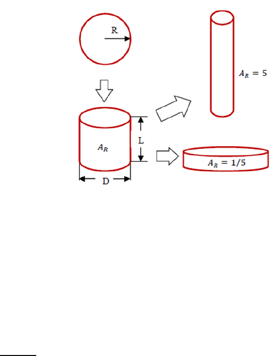
(c) Morphology evolution
The driving force for the evolution of the aspect ratio of the precipitate stems
from the anisotropic misfit strain of the precipitate and from the orientation
dependence of the interface energy. The SFFK model was modified to account
for shape factor and its evolution during precipitation process [2006Koz,
2008Svo]. In the model, the precipitate shape is approximated by a family of
cylinders having a length and a diameter as shown in Figure 5.3. The
aspect ratio
is used to describe the precipitate shape given by
. The
quantity is the equivalent precipitate radius of the spherical shape with the
same volume of the cylindrical precipitate. With this definition, small values of
represent discs, whereas large values of
represent needles as shown in
Figure 5.3.
135
Figure 5.3 Schematic plot illustrating aspect ratio
In PanPrecipitation, the aspect ratio
of a precipitate phase can be treated as
either a constant or a variable during evolution. In the former case, a set of
shape factors are calculated based on
and the growth models are adjusted
accordingly [2006Koz]. The shape factor relating the surface of the cylindrical
precipitate to the spherical precipitate is given by,
(5.19)
The shape factor for interface migration of the precipitate is given by
. The shape factor for diffusion inside the precipitate
is given by
. The shape factor for diffusion
outside the precipitate is given by
.
In the latter case, the original SFFK model was modified and the evolution
equations are described by a set of independent parameters including the
effective radius (), mean chemical composition (
) and the aspect ratio
of
each precipitate phase. The evolution rates of these parameters
are obtained by solving the linear equation
Ay B=
[2008Svo]. In the modified
SFFK, the shape evolution is determined by the anisotropic misfit strain of the

136
precipitate and by the orientation dependence of the interface energy. The total
Gibbs energy of the system, G, is given by,
(5.20)
The first term is the chemical part of the Gibbs energy of the matrix, the
second term corresponds to the stored elastic energy and the chemical part of
the Gibbs energy of the precipitates and the third term represents the total
precipitate/matrix interface energy. The subscripts ‘‘0” denote quantities
related to the matrix, e.g.,
is the number of moles of component i in the
matrix and
its chemical potential in the matrix. The quantity
accounts for the contribution of elastic strain energy due to the volume
misfit between the precipitate and the matrix and is calculated from equation
(5.6).
are the values of chemical potentials in the precipitates corresponding
to
. In the model, there are two interface energies that must be assigned:
at the mantle of the cylinder and
at the bottom and top of the cylinder. The
shape factor
is obtained by calculating equivalent radius of a
sphere
with the same volume of cylinder.
5.1.3.3 Precipitation Strengthening Model
The precipitation hardening arises from the interactions between dislocations
and precipitates. Specifically, the dispersed precipitate particles act as pinning
points or obstacles and impede the movement of dislocations through the
lattice, and therefore strengthen the material. In general, either a dislocation
would pass the obstacles by cutting through the small and weak particles (the
shearing mechanism) or it would have to by-pass the strong impenetrable
precipitates (the by-passing mechanism). The shearing mechanism is believed
to predominate in lightly aged alloys with fine coherent precipitates or zones,
137
while the by-passing mechanism is more characteristic of over-aged alloys with
coarser precipitates.
Following an usual approach to determine the critical resolved shear stress at
which a dislocation overcomes the obstacles in the slip plane, the response
equation can be derived and written as [1979Ger,1998Des],
P
MF
bL
=
(5.21)
where
M
is the Taylor factor,
F
the mean obstacle strength,
b
the Burgers
vector, and
L
the average particle spacing on the dislocation line. It has been
shown that the Friedel statistics gives fairly good results in the calculation of
the average particle spacing [1998Des]. Accordingly, this statistics is adopted
and equation (5.21) becomes [1998Des],
3/2
2
3
2
2
f
P
V
MF
R
b Gb
=
(5.22)
where
G
is the shear modulus,
a constant close to 0.5,
f
V
the particle
volume fraction and
R
the mean particle size.
The calculation of the mean obstacle strength
F
in equation (5.22) is
determined by the obstacle size distribution and the obstacle strength:
ii
i
i
i
NF
F
N
=
(5.23)
where
i
N
is the obstacle number density of the size class
i
R
and
i
F
is the
corresponding obstacle strength, which is related to the size of the obstacles
and how the obstacles are overcome (particle shearing or particle by-passing).
In the case of particle shearing for weak obstacles, a rigorous expressions of
the obstacle strength is quite complex and depends on different strengthening
138
mechanisms (e.g., chemical strengthening, modulus hardening, coherency
strengthening, ordering strengthening and so on). Therefore, we will not
consider the detailed mechanisms involved. Instead, a more general model
proposed by Gerold [1979Ger] is used in the present study and the obstacle
strength of a precipitate of radius
R
is given by,
F kGbR=
(5.24)
where
k
is a constant and
G
is the shear modulus.
On the other hand, the obstacle strength is constant and independent of
particle radius
R
in the case of particle by-passing [1979Ger],
2
2F Gb
=
(5.25)
where
is a constant close to 0.5. From equations (5.24) and (5.25), one can
find that the critical radius for the transition of the shearing and the by-
passing mechanism is
2
C
b
R
k
=
. By treating
C
R
an adjustable parameter as
suggested by Myhr et al. [2001Myh], the equations (5.24) and (5.25) can be
written as,
2
2
2 (weak particles)
2 (strong particles)
i
iC
i
C
iC
R
Gb if R R
F
R
Gb if R R
=
(5.26)
Combining equations (5.22), (5.23) and (5.26) gives the yield strength
contributed by a particle of radius
i
R
,
3/2
,
(weak particles)
(strong particles)
i
i
f
i
C
P i C
i
i
Pi
f
P i C
R
N
V
R
k if R R
N
R
V
k if R R
R
=
(5.27)
139
where
3
2
2
P
k GbM
=
. This leads to the expression for the yield strength
arising from precipitation hardening in the general case where both shearable
(weak) and non-shearable (strong) particles are present,
,P P i
i
=
(5.28)
Equations (5.27) and (5.28) yield the relationships
P
f
VR
and
P
f
V
R
,
respectively, in the two extreme case of pure shearing (i.e., all particles are
small and shearable) and pure by-passing (i.e., all particles are bigger than the
critical radius and non-shearable). The two relationships are consistent with
the usual expressions derived from the classical models.
Besides the precipitate hardening
P
, the other two major contributions
should be considered in the calculation of the overall yield: 1)
0
, the baseline
contribution including lattice resistance
i
, work-hardening
WH
and grain
boundaries hardening
GB
; 2)
SS
, the solid solution strengthening. If all three
contributions can be estimated individually, the overall yield strength of the
material can thus be obtained according to the rule of additions. Several types
of these rules have been proposed to account for contributions from different
sources [1975Koc, 1985Ard]. A general form is written as [1985Ard],
qq
i
=
(5.29)
when
1q =
, it is a linear addition rule and it becomes the Pythagorean
superposition rule when
2q =
. The value of
q
can also be adjusted between 1
and 2 in terms of experimental data. When applying to aluminum alloys, the
linear addition rule has been shown to be the appropriate one [1985Ard,
1998Des, 2001Myh, 2003Esm] and therefore the overall yield strength is given
by the following equation,
0 SS P
= + +
(5.30)

140
where
0 WH GBi
= + +
; it does not change during precipitation process.
SS
is
the solid solution strengthening term, which depends on the mean solute
concentration of each alloying element [1964Fri, 2001Myh],
2/3
SS j j
j
aW
=
(5.31)
where
j
W
is the weight percentage of the
th
j
alloying element in the solid
solution matrix phase and
j
a
is the corresponding scaling factor.
P
is the
precipitation hardening term defined by equation (5.28). By applying a
regression formula [1991Gro, 2001Myh], the yield strength
in MPa can be
converted to hardness
HV
in VPN as,
HV A B
=+
(5.32)
where A and B are treated as fitting parameters in terms of experimental data.
5.1.3.4 Precipitation hardening model with multiple particle groups
The calculation of precipitation strengthening
in equation (5.30) can be
extended to multiple particle groups with different strengthening mechanism,
(5.33)
Where is the size group defined by a particle size range and
is the volume
fraction of the group. is the strengthening mechanism in each size group.
is the weight fraction of the mechanism with
the critical radius
for transition from one mechanism to another.
141
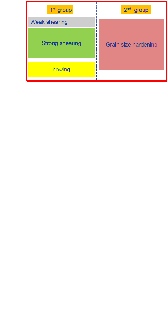
Figure 5.4 Schematic plot for strengthening groups
As an example shown in Error! Reference source not found., the first group
has three mechanisms “weak shearing”, “strong shearing” and “bowing” while
the second group has only one mechanism. This is very typical in the
strengthened Ni-based superalloys. The big primary acts to limit grain
growth during solution treatment and enhances grain boundary strengthening
while the tertiary/secondary
particles strengthen materials through the
weak/strong shearing and bowing mechanisms. In [2015Gal], Galindo-Nava
proposed an unified model for weak/strong shearing and bowing mechanisms.
The transitions from weak to strong shearing and to bowing are automatically
taken care. The unified critical resolved shear stress
is calculated as,
(5.34)
Where
is the length of the leading dislocation cutting the precipitates and
defined as,
(5.35)
with the critical radius defined as,
(5.36)

142
Where is the shear modulus and is the magnitude of the Burgers vector. In
Equation (5.34), the mean distance
is given by
with
and
.
The Orowan yield stress is given by,
(5.37)
Where is the Taylor orientation factor. The total yield strengthen due to
precipitation hardening can be calculated by equation (5.33).
5.1.4 The Precipitation Database Syntax and Examples
The precipitation database (.KDB) uses the XML format, which defines the
kinetic model for each precipitate phase and its corresponding model
parameters such as interfacial energy, molar volume, nucleation type,
morphology type, and so on.
In the KDB, a series of alloys can be defined. Each alloy has a matrix phase
with one or multiple precipitate phases. A sample kdb structure is shown as
follows,
<Alloy name="Fe-Mn-C">
<MatrixPhase name="Bcc">
<ParameterTable type="kinetic" name="Parameters for Bcc"> </ParameterTable >
<PrecipitatePhase name="Cementite_GB" phase_name="Cementite" model="kwn"
morphology="Sphere" nucleation="Grain_Boundary" growth="simp">
<ParameterTable type="kinetic" name="Parameters for Cementite">
<Parameter type="Molar_Volume" value="6E-6" description="Molar Volume" />
<Parameter type="Interfacial_Energy" value="0.2" description=
"Interfacial Energy" />
</ParameterTable >
143
</PrecipitatePhase >
<PrecipitatePhase name="M7C3_GB" phase_name="M7C3" model="kwn"
morphology="Sphere" nucleation="Grain_Boundary" growth="simp">
<ParameterTable type="kinetic" name="Parameters for M7C3">
<Parameter type="Molar_Volume" value="6E-6" description="Molar Volume" />
<Parameter type="Interfacial_Energy" value="0.1" description=
"Interfacial Energy" />
</ParameterTable >
</PrecipitatePhase >
</MatrixPhase >
</Alloy >
In this sample KDB, an alloy “Fe-Mn-C” is defined with the matrix phase “Bcc”,
which has two precipitate phases “Cementite_GB” and “M7C3_GB”. The
precipitate name, kinetic model, morphology, as well as nucleation and growth
model can be defined for each precipitate phase. Available options for the
kinetic models and morphology are given in Table 5.2. A set of parameters for
each phase, such as molar volume, interfacial energy, and so on, can be
defined in “ParameterTable”. The kinetic and mechanical model parameters
that can be defined under “ParameterTable” are listed in Table 5.3 and Table
5.4.

144
Table 5.2 Model options in kdb
Name
Options
Description
model
KWN, Fast-Acting(FA)
Refer to Figure 5.2
morphology
Sphere, Cylinder
Refer to Figure 5.3. The aspect ratio
and shape
factors are set to 1 automatically when “Sphere” is
selected.
nucleation
Modified_Homogeneous,
Grain_Boundary, Grain_Edge,
Grain_Corner, Dislocation
Refer to Table 5.1. Both homogeneous and
heterogeneous nucleation can be considered by
“Modified_Homogeneous”. In this case, the values of
and
must be manually adjusted through Nf,
Gv and GS as discussed in Table 5.3.
growth
Simplified, SFFK,
SFFK_Shape_Evolution
A constant value of The aspect ratio
can be
assigned for “Simplified” and “SFFK”. Choose
“SFFK_Shape_Evolution” for shape evolution, which
means AR varies during particle growth.
phase_name
Each “PrecipitatePhase” has a “name” and
“phase_name”. “phase_name” must be consistent
with the name in tdb/pdb. The “phase_name” tag can
be empty if “name” and “phase_name” are same.
Table 5.3 Kinetic parameter models in kdb
Name
Unit
Description
Equation
Molar_Volume
m
3
/mole
Molar volume of matrix or precipitate phase
<Parameter type="Molar_Volume" value="6E-6"
description="Molar Volume" />
in (5.2) and
in (5.3)
Grain_Size
m
The grain size of the matrix phase
<Parameter type="Grain_Size" value="1e-4"
description="Grain size, default value = 1e-4m"
/>
in (5.12)
Dislocation_Density
The dislocation density in the matrix phase
<Parameter type="Dislocation_Density"
value="1e13" description="Dislocation density,
Default value =1.0e12/m^-2" />
in (5.10)
Grain_Aspect_Ratio
N/A
The aspect ratio for the matrix grain
<Parameter type="Grain_Aspect_Ratio"
value="1.0" description="grain aspect ratio,
default value = 1.0" />
in (5.12)
Contact_Angle
degree
Contact angle of nucleus on grain boundary, default
value = 90 degree
in
(5.8)
Aspect_Ratio
N/A
The aspect ratio of the precipitate phase. The value of
is evolving if “SFFK_Shape_Evolution” is chosen as
in (5.19)

145
growth model.
<Parameter type="A_R" value="1"
description="Initial aspect ratio" />
Interfacial_Energy
2
/Jm
Interfacial energy
<Parameter type="Interfacial_Energy"
value="0.2" description="Interfacial Energy" />
User keyword “IPB_CAC(*)” to get the calculated
interfacial energy:
<Parameter type="Interfacial_Energy"
value="IPB_CALC(*)" description="Interfacial
Energy" />
in (5.2) and
(5.13)
Interfacial_Energy_L
2
/Jm
Interfacial energy in L direction
<Parameter type="Interfacial_Energy_L"
value="0.05" description="Interfacial Energy in
L direction" />
Used in
“SFFK_Shape_Evol
ution” model
Antiphase_Boundary
_Energy
2
/Jm
Antiphase boundary energy
in (5.34) and
(5.36)
Atomic_Spacing
m
Usually use lattice constant
<Parameter type="Atomic_Spacing" value="7.6E-
10" description="Atomic Spacing" />
a
in equations
(5.4)
Nucleation_Site_Para
meter
N/A
Homogeneous: choose a value close to solute
concentration;
Heterogeneous: choose a value close to nucleation density
when “Modified_Homogeneous” option is chosen for
nucleation model. Otherwise, use the model automatically
estimate the nucleation density and default value of 1.0
can be used. Such an example is given in section
5.1.4.5.
in (5.7) and
(5.11)
Driving_Force_Factor
N/A
A factor adjusting chemical driving force obtained by
thermodynamic calculation
A pre-factor
applied to
V
G
in
equation (5.2)
Strain_Energy
3
/Jm
The elastic strain energy per volume of precipitate
offsetting the calculated value by equation (5.5)
Volume_Misfit
N/A
The volume misfit
in (5.6)
Kinetic_Parameter_F
actor
N/A
A factor adjusting kinetic parameter obtained by
thermodynamic and mobility calculation
A pre-factor
applied to adjust
K
in equation
(5.14)
Effective_Diffusivity_
Factor
N/A
A factor adjusting effective diffusivity for nucleation
obtained by mobility calculation
A pre-factor
applied to adjust
in equation
(5.4)
Steady_State_Nuclea
tion_Rate
N/A
0: transient nucleation rate;
1: steady state nucleation rate;
exp( )
t
−
in
equation (5.1)

146
Table 5.4 Mechanical model parameters defined in kdb
Name
Unit
Description
Equation
Shear_Modulus
Pa
The shear modulus of the matrix phase
in (5.6) and (5.36)
Burgers_Vector
m
The Burgers vector of the matrix phase
in(5.36)
Taylor_Factor
N/A
The Taylor factor of the matrix phase
in (5.37)
Solution_Strengthening
_Factor
N/A
scaling factor of alloying element for solution
strengthening
j
a
in equation (5.31)
Strength_Parameter
N/A
Strengthening parameter due to precipitation
hardening
P
k
in equation (5.27)
Shearing_Critical_Radi
us
m
Critical radius shifting from shearing to looping
mechanism
C
R
in equation (5.27)
Intrinsic_Strength
MPa
The baseline contribution including lattice resistance,
work-hardening and grain boundaries hardening.
0
in equation (5.30)
Hardness_Factor
N/A
The yield strength in MPa can be converted to
hardness in VPN based on eq (5.31)
A in equation (5.32)
Hardness_Constant
VPN
The yield strength in MPa can be converted to
hardness in VPN based on eq (5.31)
B in equation (5.32)
Table 5.5 Symbol and syntax for retrieving system quantities
Name
Unit (SI)
Comments
time
second
Time
T
K
Temperature
vft
Total Transformed Volume Fraction:
p
p
vft vf=
where
p
vf
is the transformed volume fraction of
p
phase
x(comp), w(comp)
Overall alloy composition
Table 5.6 Symbol and syntax for retrieving quantities of precipitate phases
Name
Unit (SI)
Comments
s(@phase)
m
Average size/radius of equivalent sphere particles

147
D(@phase)
m
Diameter of cylinder
L(@phase)
m
Length/Height of cylinder
A_R(@phase)
m
Aspect ratio of cylinder
nd(@phase)
#m
-3
Number density
nr(@phase)
m
-3
sec
-1
Nucleation rate
vf(@phase)
Volume fraction of specified phase
x(comp@phase),
w(comp@ phase)
Instant composition of the matrix or precipitate
phases
IPB_CALC(@phase)
J/m
2
Model calculated interfacial energy
dgm(@phase)
J/mole
Nucleation driving force of phase(s)
vf_range(@phase,lb,ub)
The volume fraction for different particle groups
defined by a size range [lb, ub] such as primary,
secondary and tertiary in Ni-based super alloys, for
example vf_range(@L12_FCC,0.5e-8, 0.5e-7)
s_range(@phase,lb,ub)
average size for different particle groups defined by a
size range [lb, ub], for example
s_range(@L12_FCC,0.5e-8, 0.5e-7)
Table 5.7 Symbol and syntax for retrieving quantities of particle size
distribution (PSD)
Name
Unit
Comments
time
The PSDs are saved for the user-specified times; the PSD for
the last time step is automatically saved. Using time = t to
get the PSD for time “t”.
psd_id
The PSD consists of a certain number of cells (size classes);
psd_id gets the cell id.
psd_s(@phase)
m
The characteristic size of a precipitate phase for each cell.

148
psd_nd(@phase)
#m
-3
The number density of a precipitate phase for each cell.
psd_gr(@phase)
m/sec
The growth rate of a precipitate phase for each cell.
psd_ns(@phase)
Normalized size of the cell
psd_nnd(@phase)
Normalized number density of the cell
psd_df(@phase)
The distribution function:
with being the
cell width
psd_cvf(@phase)
Cumulative volume fraction of phase(s). Example:
psd_cvf(@L12_FCC).
Table 5.8 Symbol and syntax for retrieving mechanical properties
Name
Unit (SI)
Comments
sigma_y
MPa
Overall yield strength. Example: sigma_y
hv
vpn
Overall microhardness. Example: hv
sigma_i
MPa
Intrinsic yield strength. Example: sigma_i.
sigma_ss
MPa
Yield strength due to solution strengthening. Example:
sigma_ss.
sigma_p(@*)
MPa
Yield strength due to precipitation hardening. Example:
sigma_p(@Mg5Si6).
Table 5.9 Constants of mathematics and physics
Name
Comments
_K
Boltzmann constant
_PI
Archimedes' constant.
_R
Molar gas constant.

149
_NA
Avogadro constant.
_E
Natural Logarithmic Base.
Table 5.10 Mathematical operators
Name
Comments
+
Addition
-
Subtraction
*
Multiplication
/
Division
^
Exponentiation
Table 5.11 Mathematical Functions
Name
Comments
exp(x)
Exponential
ln(x)
Natural Logarithm of x
log2(x)
Base 2 Logarithm of x
log10(x)
Base 10 Logarithm of x
sqrt(x)
Square root of x
abs(x)
Absolute value of x
sin(x)
Sine of x
cos(x)
Cosine of x
tan(x)
Tangent of x

150
asin(x)
Inverse sine of x
acos(x)
Inverse cosine of x
atan(x)
Inverse tangent of x
A few examples are given below to explain the content of the precipitation
database in detail. In the reference folder, test batch files (.pbfx) are prepared
with .kdb files for running example simulations.
5.1.4.1 An example kdb file for Ni-14Al (at%) alloy
Reference Folder: $Pandat_Installation_Folder\Pandat 2020 Examples
\PanPrecipitation\Ni-14%Al\Ni-14Al_Precipitation.kdb
This precipitation database defines the kinetic parameters for the L1
2
_Fcc (γ’)
phase in the Ni-Al binary system at the Ni-rich side. The matrix phase is
Fcc_A1 (γ) phase. The detail explanations of kinetic parameters are listed in
Table 5.3. This precipitation database can be used for multi-component Ni-
based superalloys as well, but some of the key parameters, such as the
interfacial energy, and/or nucleation site parameter, may need to be calibrated
accordingly. The molar volume and atomic spacing for various types of crystal
structures can be found or estimated following reference of ASM handbook.
The interfacial energy between γ and γ’ for nickel alloys is usually in the range
of 0.02-0.035 J/m
2
, it is given as a constant in this example. Interfacial energy
can be estimated as discussed in 5.1.3.1(c), and an example is given in the
following section 5.1.4.2.
<Alloy name="NI-14Al_KWN">
<MatrixPhase name="Fcc">
<ParameterTable type="kinetic" name="Parameters for gamma">
<Parameter type="Molar_Volume" value="7.1E-6" description="Molar Volume" />
</ParameterTable >

151
<PrecipitatePhase name="L12_FCC" model="KWN" morphology="Sphere"
nucleation="Modified_Homo" growth="SFFK">
<ParameterTable type="kinetic" name="Parameters for Gamma_prime">
<Parameter type="Molar_Volume" value="7.1E-6" description="Molar Volume" />
<Parameter type="Interfacial_Energy" value="0.025" description=
"Interfacial Energy" />
<Parameter type="Atomic_Spacing" value="3.621E-10" description=
"Atomic Spacing" />
<Parameter type="Nucleation_Site_Parameter" value="0.001" description=
"Nucleation Site Parameter" />
</ParameterTable >
</PrecipitatePhase >
</MatrixPhase >
</Alloy >
5.1.4.2 An example kdb file for Ni-14Al (at%) alloy using the calculated
interfacial energy
Reference Folder: $Pandat_Installation_Folder\Pandat 2020 Examples
\PanPrecipitation\Ni-14%Al_IPB_CALC\Ni-14Al_Precipitation.kdb
In .kdb file, use keyword “IPB_CALC(*)” to get the calculated interfacial energy.
The value can also be an expression, such as: value="1.2 * IPB_CALC(*)".
The optional parameter “Interfacial_Energy_Tc” is used to define the
temperature at which γ’ forms from γ congruently, and
represents the
congruent point. In many cases this point does not exist. This parameter is
optional and users should not give an arbitrary value to this parameter since it
will lead to unrealistic results. In this example, this parameter is commented
out in the Ni-14Al_Precipitation.kdb kinetic database. This means the
correction factor
in Eq. (5.13) is set to be 1.
<Parameter type="Interfacial_Energy" value = "IPB_CALC(*)" description =

152
"Interfacial Energy" />
5.1.4.3 An example kdb file for AA6005 Al alloy
Reference Folder: $Pandat_Installation_Folder\Pandat 2020 Examples
\PanPrecipitation\AA6005_yield_strength\AA6xxx.kdb
This precipitation database defines the kinetic parameters for the Mg
5
Si
6
(’)
phase within the Al-Mg-Si alloys at the Al-rich side. The matrix phase is
Fcc_A1-(Al) phase. This example AA6xxx.kdb can be used for most of the
AA6xxx and AA3xx series of alloys. Again, some of the key kinetic parameters
may need to be slightly revised according to the chemical compositions. Note
that, the strengthening model is also included, which enables us to simulate
the yield strength (σ) as well as its contributions (σ
i
, σ
ss
, σ
p
). Using the equation
(5.30), the hardness can then be obtained as well. Table 5.4 lists the
strengthening model parameters defined in the precipitation database. These
model parameters are adjustable and obtained via optimization to describe
available experimental data.
<Alloy name="AA6xxx">
<MatrixPhase name="Fcc">
<ParameterTable type="Strength" name="Parameters for Fcc">
<Parameter type="Solution_Strengthening_Factor" name="Si" value="66.3"
description="solid solution strengthening scaling factor" />
<Parameter type="Solution_Strengthening_Factor" name="Mg" value="29"
description="solid solution strengthening scaling factor" />
<Parameter type="Solution_Strengthening_Factor" name="Cu" value="46.4"
description="solid solution strengthening scaling factor" />
<Parameter type="Solution_Strengthening_Factor" name="Li" value="20"
description="solid solution strengthening scaling factor" />
<Parameter type="Intrinsic_Strength" value="10" description=
"intrinsic strength" />
153
<Parameter type="Hardness_Factor" value="0.33" description=
"intrinsic strength" />
<Parameter type="Hardness_Constant" value="16" description=
"intrinsic strength" />
</ParameterTable >
<ParameterTable type="kinetic" name="Parameters for (Al)">
<Parameter type="Molar_Volume" value="1.0425E-5" description=
"Molar Volume" />
</ParameterTable >
<PrecipitatePhase name="Mg5Si6" model="KWN" morphology="sphere"
nucleation="Modified_Homo" growth="SFFK">
<VariableTable name="Variables replacing built-in variables">
<Parameter type="Nucleation_Barrier_Energy" value="7.475e-12/dgm(*)^2"
description="Nucleation_Barrier_Energy" />
</VariableTable >
<ParameterTable type="kinetic" name="Parameters for kinetic model">
<Parameter type="Molar_Volume" value="3.9e-5"
description="Molar Volume" />
<Parameter type="Interfacial_Energy" value="0.4"
description="Interfacial Energy" />
<Parameter type="Atomic_Spacing" value="4.05E-10"
description="Atomic Spacing" />
<Parameter type="Nucleation_Site_Parameter" value="0.3e-5"
description="Nucleation Site Parameter" />
<Parameter type="Steady_State_Nucleation_Rate" value="1"
description="Indicate whether or not steady state nucleation rate" />
<Parameter type="Driving_Force_Factor" value="1.0"
description="Driving Force Factor" />

154
<Parameter type="Kinetic_Parameter_Factor" value="3.0"
description="a factor for kinetic parameter" />
<Parameter type="Effective_Diffusivity_Factor" value="3"
description="a factor for effective diffusivity" />
</ParameterTable >
<ParameterTable type="strength" name="Parameters for
strengthening models">
<Parameter type="Strength_Parameter" value="1.1e-5"
description="th k_ppt in the equation" />
<Parameter type="Shearing_Critical_Radius" value="5.0e-9"
description="Critical size of shifting from shearing to looping" />
</ParameterTable >
</PrecipitatePhase >
</MatrixPhase >
</Alloy >
5.1.4.4 An example for heterogeneous nucleation:
Reference Folder: $Pandat_Installation_Folder\Pandat 2020 Examples
\PanPrecipitation\AA6005_yield_strength\AA6xxx.kdb
There are two parameters need to be adjusted in order to consider
heterogeneous nucleation. In this example, the heterogeneous nucleation sites
and barrier energy are adjusted manually by user:
(a) Nucleation_Site_Parameter; in the above example of AA6005 alloy, the value
of 0.3e-5 was chosen based on experimental data.
(b) Re-define the nucleation barrier energy. In this example, the nucleation
barrier energy for the heterogeneous nucleation is manually adjusted. For
homogeneous nucleation, the nucleation barrier energy is defined by
equation (5.2) with
155
Taking Vm=3.9e-5 and =0.4 in the kdb file as shown in section 5.1.4.3,
we get the nucleation barrier energy for the homogeneous nucleation as
1.63e-9/ dgm(*)^2. For heterogeneous, the nucleation barrier energy is ~2-
3 order smaller than that of homogeneous nucleation. In this example, a
value “7.475e-12/dgm(*)^2” is used. This value is optimized by using
experimental data.
<VariableTable name="Variables replacing built-in variables">
<Parameter type="Nucleation_Barrier_Energy" value="7.475e-12/dgm(*)^2"
description="Nucleation_Barrier_Energy"/>
</VariableTable >
Where dgm(*) is the calculated thermodynamic driving force, which will be
update at every simulation steps.
5.1.4.5 Another example for heterogeneous nucleation:
Reference Folder: $Pandat_Installation_Folder\Pandat 2020 Examples
\PanPrecipitation\Fe-Mn-C_Heterogeneous_Nucleation\PanFe.kdb
In the example of section 5.1.4.4, the heterogeneous nucleation sites and
nucleation barrier energy were treated as adjustable parameters and were
given manually by the user based on available experimental data. In this
example, the potential heterogeneous nucleation sites and nucleation barrier
energy are estimated by theoretical models as discussed in section 5.1.3.1(b)
depending on the selected nucleation type.
<PrecipitatePhase name="Cementite_GB" phase_name="Cementite" model="kwn"
morphology="Sphere" nucleation = "Grain_Boundary" growth="simp">
<PrecipitatePhase name="Cementite_Dislocation" phase_name="Cementite"
model="kwn" morphology="Sphere" nucleation="Dislocation" growth="simp">

156
The nucleation type can be specified when defining a precipitate phase. In this
example, two different type of heterogeneous nucleation are defined for
“Cementite” phase: one at “Grain_Boundary” and the other at “Dislocation”.
5.1.4.6 An example kdb file for a Mg-based AZ91 alloy considering
shape factor and shape evolution
Reference Folder: $Pandat_Installation_Folder\Pandat 2020 Examples
\PanPrecipitation\AZ91_Morphology\AZ91.kdb
✓ Consider shape factor but shape factor not evolve (AZ91_200C.pbfx)
<PrecipitatePhase name="ALMG_GAMMA" model="kwn"
morphology="Cylinder" nucleation="Modified_Homo" growth="sffk">
In this case, the morphology must be set to “morphology="Cylinder"” and the
keyword “Aspect_Ratio” or “A_R” is used to set the aspect ratio of the particles:
<Parameter type="A_R" value="0.15" description="aspect ratio" />
In this example, the Aspect Ratio is set as a constant during the particle
evolution.
✓ Shape evolution (AZ91_200C_shape_evolution.pbfx)
<PrecipitatePhase name="ALMG_GAMMA" model="KWN" morphology="Cylinder"
nucleation="Modified_Homo" growth="SFFK_Shape_Evolution">
In order to consider shape evolution, the morphology must be set to
“morphology="Cylinder"” and the growth model should be set to
“growth="SFFK_Shape_Evolution"”.
In this case, the aspect ratio value set in “<Parameter type="A_R"
value="1" description="Initial aspect ratio" />” will be used as a
starting value and evolves during precipitation process.
There are two sets of parameters that can control the shape evolution. The first
set includes the interfacial energies of the two different directions:
<Parameter type="Interfacial_Energy" value="0.25" description=

157
"Interfacial Energy" />
<Parameter type="Interfacial_Energy_L" value="0.05" description=
"Interfacial Energy in L direction"/>
The second set includes the anisotropic misfit strain of the precipitate and its
model parameters can be defined as follows:
<Parameter type="Shear_Modulus" value="30e9" description=
"the shear modulus, in Pa"/>
<Parameter type="Volume_Misfit" value="0.02" description=
"the volume misfit"/>
It should note that user can set parameters for either interfacial energy or
strain energy or both to control the shape evolution.
5.1.4.7 An example to show how to set an initial microstructure for
simulation
Reference Folder: $Pandat_Installation_Folder\Pandat 2020 Examples
\PanPrecipitation\Ni-16%Al_Dissolution\Al-Ni.ini
This example is to demonstrate how to set up the initial microstructure for
dissolution simulation. In this example, the alloy composition is Ni-16Al at.%,
which is isothermally annealed at 1444K for 100 seconds. The alloy
composition and heat treatment condition is given in Ni-16Al_dissolution.pbfx.
Initially, there is 10% (volume fraction) L1
2
_Fcc (’) phase with average particle
size 1.2µm. The initial microstructure is set in Al-Ni.ini as shown below:
<Condition name="C1">
<MatrixPhase name="Fcc">
<PrecipitatePhase name="L12_FCC">
<Parameter name="size" value="1.2e-6" description="average size" />
<Parameter name="volume_fraction" value="0.1" description=
"volume fraction" />
<Parameter name="particle_size_distribution" value="2" number_cells =
158
"200" sigma="0.25" description="initial psd shape: 0-uniform;
1-normal; 2-lognormal;10: user-defined psd" />
<psd>
<cell size="1.2E-08" number_density="170191212760.267" />
<cell size="2.4E-08" number_density="199242482086.767" />
<cell size="3.6E-08" number_density="232879833831.677" />
<cell size="4.8E-08" number_density="271760886495.754" />
<cell size="6E-08" number_density="316626417716.63" />
……
</psd>
</PrecipitatePhase >
</MatrixPhase >
</Condition>
The “<psd> ” section can be empty if uniform, normal or lognormal distribution
is selected and the initial PSD is automatically generated based on the defined
number_cells and standard deviation sigma. If the “<psd> ” section is given,
the provided psd data will be used and the defined initial psd shape (uniform,
normal or lognormal distribution) is neglected.
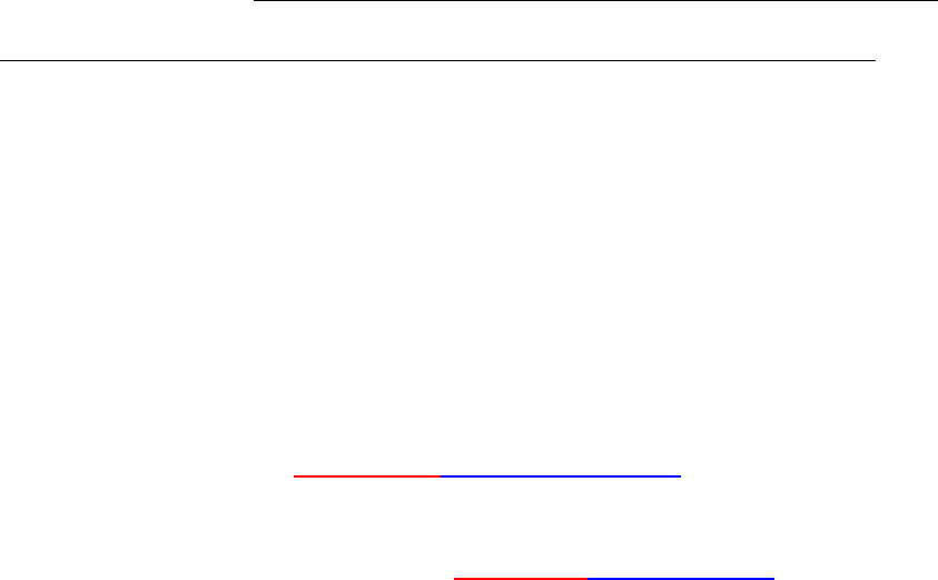
User can also define the initial structure from GUI. User first chooses the target
phase to set the initial structure and then set the average quantities including
the volume fraction and average size. The PSD type can be “uniform”, “normal”,
“log_normal” or “user_defined”. When “normal” and “log_normal” are selected,
the PSD data will be generated and the corresponding plot is shown on the
right panel. In order to load a user defined PSD, the user can set PSD type to
be “user_defined” and then load the PSD data file by clicking the import button.
An example PSD data file “psd_test.dat” can be found in the folder:
$Pandat_Installation_Folder\Pandat 2020 Examples\PanPrecipitation\Ni-
16%Al_Dissolution\.
159
Figure 5.5 Dialog to define the initial structure from GUI
160
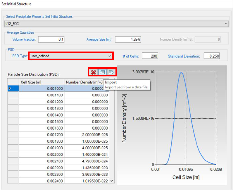
5.2 PanPrecipitation Functions
The current version of PanPrecipitation menu includes the following major
functions: Load Precipitation Database, Select Alloy Parameter,
Precipitation Simulation,and TTT Simulation.
Figure 5.6 Menu functions of PanPrecipitation
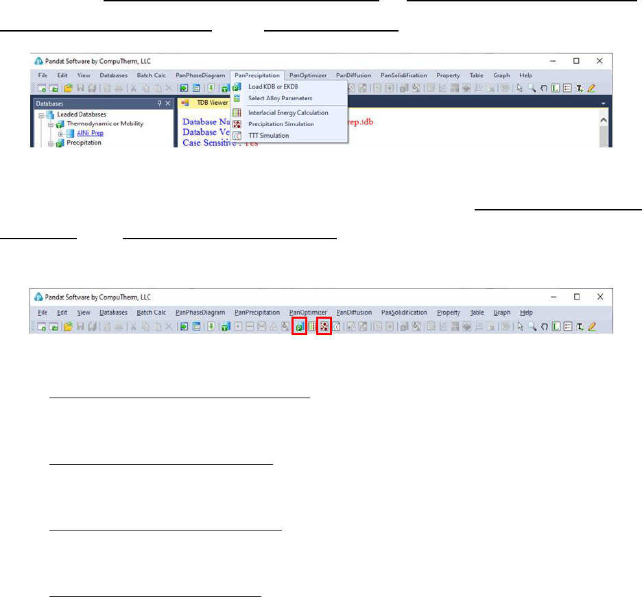
The shortcut of the two commonly used functions Load Precipitation
Database and Precipitation Simulation are also displayed in the Toolbar as
shown in Error! Reference source not found..
Figure 5.7 Toolbar buttons of PanPrecipitation
➢ Load Precipitation Database: Load a precipitation database into
PanPrecipitation module for simulation.
➢ Select Alloy Parameters: Select an alloy parameter available in
precipitation database for simulation.
➢ Select Precipitate Phases: Select one or more precipitate phases
available in precipitation database for simulation.
➢ Precipitation Simulation: Perform the precipitation simulation.

161
5.3 Tutorial
In this tutorial, the Ni -14 at% Al alloy is taken as an example to demonstrate
the functionalities provided by PanPrecipitation. The four files mentioned in
this section (“AlNi_Prep.tdb”, “Ni-14Al_Precipitation.kdb”, “Ni-
14Al_Exp.dat” and “Ni-14Al_Precipitation.pbfx”) can be found in the
installation folder of Pandat. In general, user should follow four steps to carry
out a precipitation simulation:
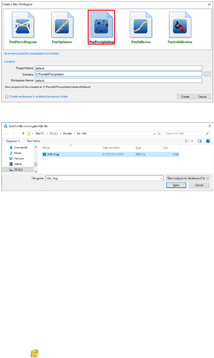
5.3.1 Step 1: Create a Workspace
Let’s start this tutorial by “creating a workspace”. By clicking the button on
the toolbar, the “Create a New Workspace” popup window will open. User can
choose the “PanPrecipitation” icon and define the location (project name,
directory and/or workspace name), then click the “Create” button to create a
precipitation workspace. User can also create a default precipitation workspace
by double-click the “PanPrecipitation” icon as shown in Error! Reference
source not found..
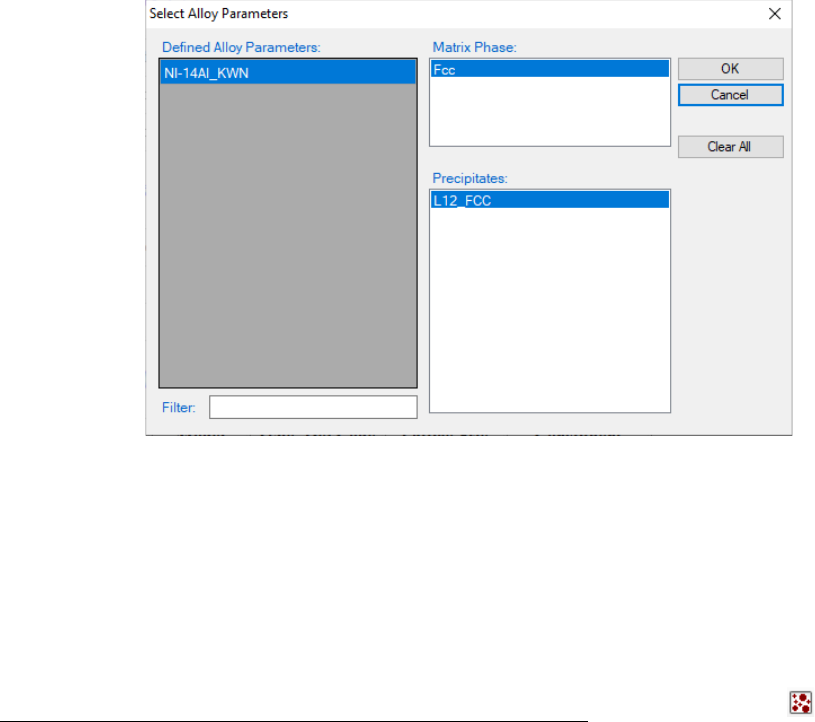
5.3.2 Step 2: Load Thermodynamic and Mobility Database
The next step is to load the database, which is AlNi_Prep.tdb in this example.
Different from the normal thermodynamic database, this database also
contains mobility data for the matrix phase (Fcc) in addition to the
thermodynamic model parameters. Both are needed for carrying out
precipitation simulation. By clicking the button on the toolbar, a popup
window will open, allowing user to select the database file. User may select the
TDB file and click on Open button or just double click on the TDB file to load it
into the PanPrecipitation module as shown in Error! Reference source not
found..
162
Figure 5.8 Dialog window for creating a workspace
Figure 5.9 Dialog window for loading thermodynamic and mobility database
5.3.3 Step 3: Load Precipitation Database
A precipitation database is required for precipitation simulation. Such a
database contains kinetic parameters which are alloy dependent. Each alloy is
composed of one matrix phase and a number of precipitate phases. To organize
these parameters in a more intuitive way, the standard XML format is adopted
and a set of well-formed tags are deliberately designed to define the kinetic
model (KWN or Fast_Acting) for each precipitate phase and its corresponding
model parameters such as interfacial energy, molar volume, nucleation type,
and morphology type.
In this example, the Ni-14Al_Precipitation.kdb is prepared. This file can be
opened by click button in the toolbar and be viewed in the Pandat
workspace or through third-party external editors, such as NotePad, WordPad
etc. The advantage to open this file in Pandat workspace is that all the key

163
words will be highlighted which makes it easy to read. In this example, the
matrix phase for this alloy is “Fcc”, which has one precipitate phase “L12_FCC”.
The “KWN” model with “Sphere” morphology and “Modified Homogeneous”
nucleation type are selected for precipitation simulation. There are five model
parameters: Molar_Volume, Interfacial_Energy, Atomc_Spacing,
Nucleation_Site_Parameter, and Driving_Force_Factor. These parameters have
been developed for the Ni-14Al alloy in this particular example; these
parameters need to be optimized for different alloys in terms of experimental
data.
Please note that, two sets of model parameters are given in the Ni-
14Al_Precipitation.kdb file for two models: KWN or Fast_Acting models. User
may select either one for the simulation as is shown in Error! Reference
source not found..
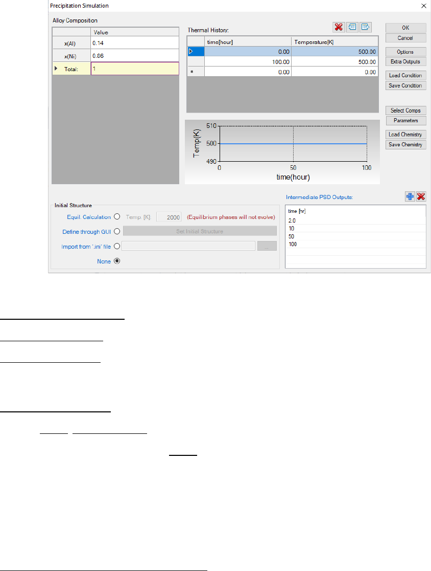
To load a precipitation database, user should navigate the command through
menu PanPrecipitation → Load Precipitation Database, or click icon
from the toolbar. After Ni-14Al_Precipitation.kdb is chosen, a dialog box pops
out automatically for user to select the model, i.e., Ni-14Al_FAST or Ni-
14Al_KWN, for the simulation. As shown in Error! Reference source not
found., the “Ni-14Al_KWN” is chosen in this example. The Matrix Phase
window allows user to select the matrix phase and the Precipitates window
allows user to choose one or more precipitate phases of interest for simulation.
To select several phases at one time, press and hold the <Ctrl> key.
164
Figure 5.10 Dialog box for selecting alloy parameter
5.3.4 Step 4: Precipitation Simulation
After successfully loading both thermodynamic/mobility and precipitation
databases, the function for precipitation simulation is then being activated. To
perform a precipitation simulation, choose from Pandat GUI menu
PanPrecipitation → Precipitation Simulation, or click icon from the
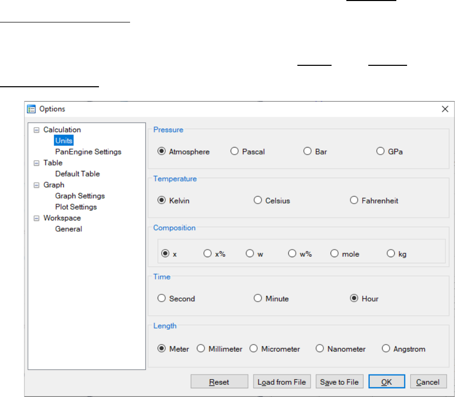
toolbar. A dialog box entitled “Precipitation Simulation”, as shown in Figure
5.11, pops out for user’s inputs to set up the simulation conditions: alloy
composition and thermal history.
165
Figure 5.11 Dialog box for setting precipitation simulation conditions
Alloy Composition: User can set alloy composition by typing in or use the
Load Chemistry function. User can also save the alloy composition through
Save Chemistry. This is especially useful when working on a multi-component
system, so that user does not need to type in the chemistry every time.
Thermal History: Arbitrary heat treatment schedule can be inputted, with a
linear Time-Temperature relationship (i.e., constant cooling or heating rate) at
each two consecutive rows. Time at the first row must be zero representing the
initial time. The thermal history set up in the Figure 5.11 represents an
isothermal heat treatment for 100 hours at 500C. If the temperatures in the
two rows are different, it represents constant cooling or heating. Multi-stages of
heat treatment can be set by adding more rows in the Thermal History column.
Set intermediate PSD outputs: Based on the specified intermediate PSD
outputs, psd tables are automatically generated and the psd plot for the final
time step will be created. As shown in Figure 5.11, the intermediate PSD
outputs are set up at 2, 10, 50, and 100 hours, respectively.
166
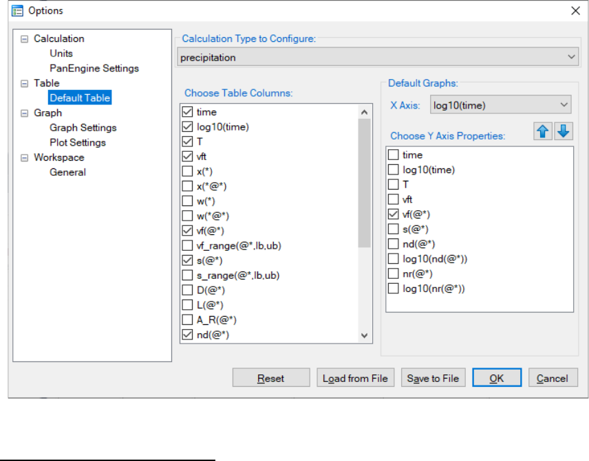
User can access the Options window by clicking the Options button. The
Calculation Options window allows user to change the units for pressure,
temperature, time and composition required in the simulation (as shown in
Figure 5.12). User can also define the output Table and Graph within the
Output Options window (as shown in Figure 5.13).
Figure 5.12 Dialog box for setting simulation units
167
Figure 5.13 Dialog box for setting simulation outputs
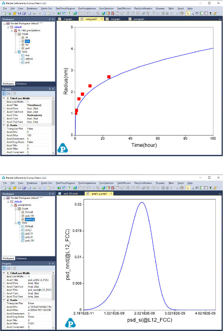
In Precipitation Simulation window (as shown in Figure 5.11), click OK to
run the simulation. After the simulation is completed, its results are displayed
in two types of formats in the Pandat
TM
Explorer window: Graph and Table. By
default, the graphs plotting average size evolution and PSD at 100 hours are
displayed in the Pandat
TM
main window as shown in Figure 5.14 and Figure
5.15, respectively. To view detailed simulation results, user can switch from
Graph view to Table View by clicking tabs in the Pandat
TM
Explorer window.
168
Figure 5.14 Default graph plotting average size changes
Figure 5.15 Calculated PSD at 100 hour
User can customize the output results with Pandat batch file. Experimental
data may be imported as a separate table using the syntax below:

169
<table source="Ni-14Al_Exp.dat" name="exp"/>
The experimental data file should be in the same folder where the batch file
locates, otherwise a full path is needed for the experimental file as shown
below:
<table source="D:\Pandat\Precipitation\Ni-14Al_Exp.dat" name="exp"/>
And the experimental data can be plotted together with the calculated results
using the syntax below to obtain a diagram as shown in Figure 5.14.
<graph name="size">
<plot table_name="default" xaxis="t/3600" yaxis="s(*)*1e9"/>
<plot type="point" table_name="exp" xaxis="t(hr)" yaxis="radius(nm)"/>
</graph>
5.3.5 Step 5: Customize Simulation Results
As all other calculations available in Pandat
TM
, upon the completion of the
precipitation simulation, a default table with related kinetic properties (such as
time, total transformed volume fraction, average size of each precipitate phase,
number density of each precipitate phase and nucleation rate of each
precipitate phase) is automatically generated and a default graph for average
size changes is displayed Figure 5.15.
However, it should be emphasized that, in addition to the default tables, variety
of properties, such as temperature, volume fraction of each individual
precipitate phase, instant composition of matrix phase and also size
distribution related information if the KWN model is used for simulation, can
be retrieved through “Add a new table”.
5.3.6 Add a new table
Add a new table function can be activated by the following ways: (1) selecting
the “Table” node in the Explore Window, then right click the mouse and select
“Add a New Table” option (as shown in Figure 5.16); or (2) choose “Add or Edit
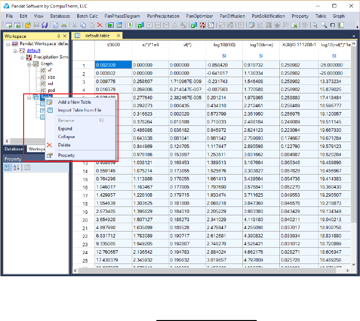
170
a Table” from the “Table” menu. This function allows user to create a new table
at their own choices.
Figure 5.16 Dialog of add a new table
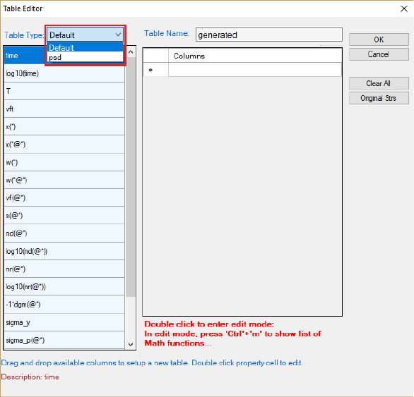
The basic layout of the window of “Add a new table” is shown in Figure 5.17.
There are two major parts in this window. The left part is the available
variables and contents. User first chooses the type of the tables from the “Table
Type” drop-down list as highlighted in Figure 5.17, to show the list of available
variables. The right part is the generated table field. User can drag the available
variables from the left column to the right side by clicking and holding the left
mouse button.
171
Figure 5.17 Dialog window of table editor
5.3.7 Table Format Syntax
Moreover, mathematical calculation over these properties is allowed in
PanPrecipitation. Accordingly, a variety of property diagrams can be generated
based on the customized tables, which offers users an excellent flexibility for
different applications. A detailed description of table format is given below.
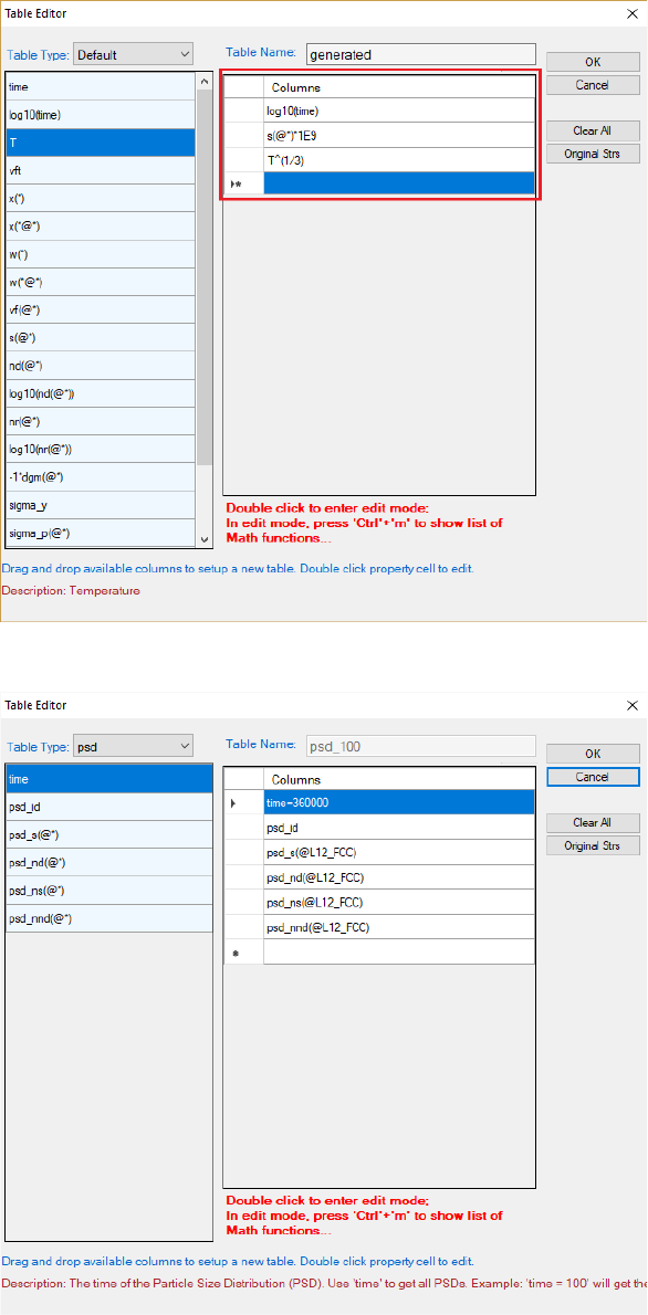
Figure 5.18 shows the dialog window of table editor for customized new table.
The symbol “*” can be used to get quantities of all the phases or all components.
As an example, s(*) retrieves the average size of phase L12_FCC, which is
equivalent to s(L12_FCC).
Figure 5.19Figure 5.19 shows the dialog window of table editor for user to get a
psd table by specifying time. For example, the psd table at 100 hours can be
obtained by setting “time = 360000”. Note that the default unit for time is
second.
172
Figure 5.18 Dialog window of table editor for customized new table
Figure 5.19 Dialog to get a psd table at a specified time