199

7 PanSolidification

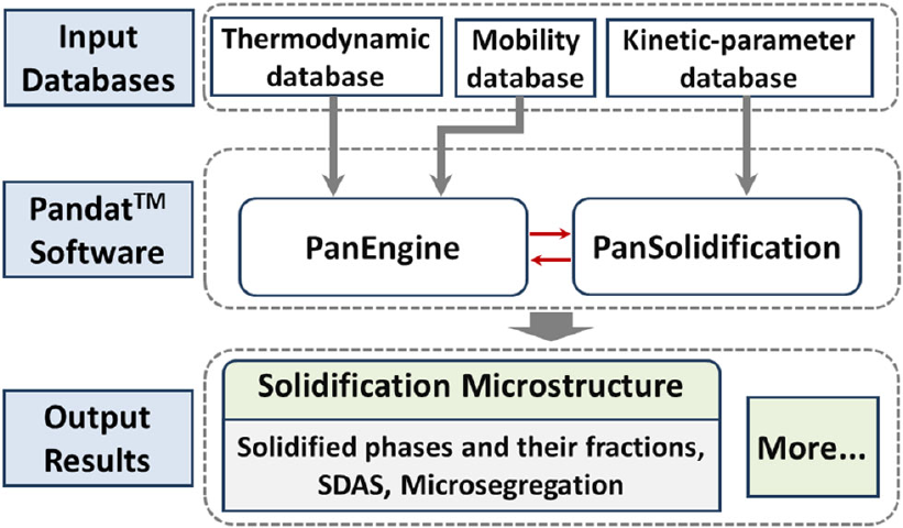
PanSolidification is a module of Pandat

software designed to simulate

solidification behavior under a variety of conditions with different cooling rates.

It is an extension of the Scheil model taking into consideration of back

diffusion in the solid, secondary dendrite arm coarsening, and the formation of

eutectic structure.

It is seamlessly integrated with the user-friendly Pandat

Graphical User

Interface (PanGUI) as well as thermodynamic calculation engine, PanEngine.

The implementation of PanEngine guarantees reliable input data, such as

chemical potential, phase equilibrium and mobility. Figure 7.1 shows an

overall architecture of the PanSolidification module.

Figure 7.1 An overall architecture of the PanSolidification module

200

7.1 Features of PanSolidification

7.1.1 Overall Design

➢ The system composition profile, phase fraction, and phase concentration

evolution during solidification

➢ Secondary dendrite arm spacing (SDAS) evolution during solidification.

➢ Back diffusion during the entire solidification process.

7.1.2 Data Structure

Thermodynamic and mobility parameters are stored in TDB file, and the kinetic

parameters for undercooling and coarsening effects are stored in an SDB file in

“Extensible Markup Language” (XML) format, which is a standard markup

language and well-known for its extendibility. In accordance with the XML

syntax, a set of well-formed tags are specially designed to define the back

diffusion model for the morphology of primary phase and its corresponding

model parameters such as interfacial energy, latent heat, coarsening geometric

factor, dendrite tip factor, solute trapping parameter, solid diffusivity factor and

boundary layer factor.

7.1.3 Numerical Model

The PanSolidification module, which is developed by coupling a solidification

micro-model with PanEngine, is basically a modified Scheil model incorporating

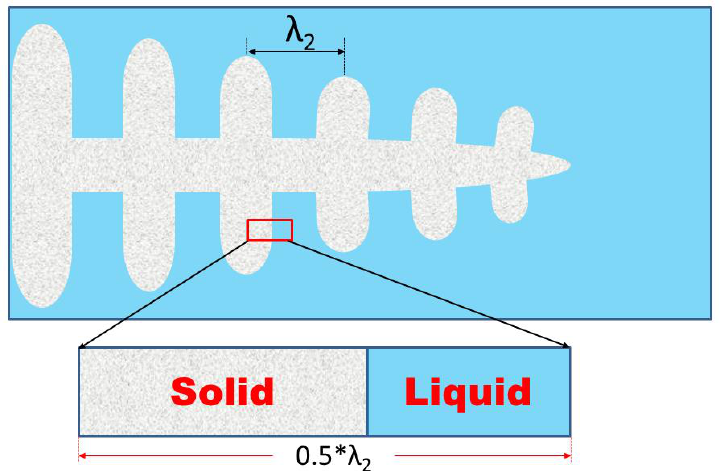
back-diffusion, undercooling, and dendrite arm coarsening. Figure 7.2 shows a

sketch of dendrite, with a big solid trunk as the primary dendrite arm and fine

secondary dendrite arms symmetrically distributed at the sides; the SDAS is

indicated as λ

. A one-dimensional morphology within the interdendritic region

of secondary arms is usually used to describe the solidification processing (as

enlarged and shown at the bottom part of Figure 7.2). Because of the symmetry

of the dendrite arms, there is no mass flow through the arm center. Therefore,

only one half of the arm spacing is considered.

201

Figure 7.2 A schematic diagram of dendrites in the solid and liquid region

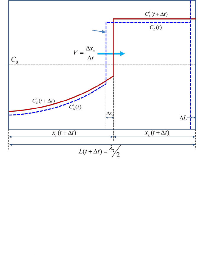
7.1.3.1 Back diffusion in the solid

The evolution of the concentration profile for component i in the considered

dendrite arm is shown schematically in Figure 7.3.

and

are compositions

of component i within the liquid and solid phases (given the unit of wt.% in this

work), respectively. V is the velocity of S/L interface. During the time interval Δt,

the S/L interface advances Δx

(due to solidification) and the length of the

solidification region increases by ΔL (due to the SDAS coarsening). For the

current solidification simulation at each time step, three major tasks are

carried out: (1) calculate the composition of each component at the S/L

interface including the undercooling effects and local-equilibrium conditions; (2)

solve the diffusion equations within the solid phase; (3) update the length scale

to conserve mass balance for every component. More detailed description on

the back diffusion can be found in some textbooks [1974Fle, 1985Kur].

202

Figure 7.3 A schematic plot showing the composition distribution of component

i in a dendrite arm at time t and t+Δt.

7.1.3.2 Micro-model for dendrite arm coarsening

The initial SDAS is about twice of the dendrite tip radius:





and

described as a function of initial alloy composition, growth rate, and

independent of temperature gradient

V T k H





(7.1)

where V, ΔT

, k

are the interface solidification velocity, freezing temperature

range, and equilibrium partition coefficient, respectively. δ is a constant being

dependent on the harmonic of the perturbation.

The dendrite arm spacing needs to be known since it sets the diffusion

distances in the liquid and solid phases. Owing to the re-melting and re-

solidification mechanism, dendrite arm coarsening contributes significantly to

homogenization during solidification. The calculation of coarsening is described

as below [1986Roo]:

203

gMdt



−=



(7.2)



is the initial SDAS obtained from the calculated dendrite tip radius as

described in above equation 7.2, and



is the model predicted SDAS at a

certain time. M is coarsening parameter which is proportional to

1/3



, t is time

and g is the geometry factor representing the influence of the dendrite geometry.

For a binary system, the coarsening parameter M is defined as [1990Roo]:

(1 )

f L v L

H m k C



−

(7.3)

For a multicomponent system, the coarsening parameter must be calculated

separately for each alloying element. Then, the following model is used to take

into consideration all the solute elements:



(7.4)

All phase equilibrium related quantities needed in the above equations (such as

and k

) are directly calculated via PanEngine [2009Cao] at each time step by

assuming the local equilibrium at the liquid/solid interface.

7.1.4 The Solidification Kinetic Database Syntax and

Examples

The Solidification kinetic database (.SDB) uses the XML format, which defines

the back diffusion model for the morphology of primary phase and its

corresponding model parameters such as interfacial energy, latent heat,

coarsening geometric factor, dendrite tip factor, solute trapping parameter,

solid diffusivity factor, boundary layer factor, and so on.

In the SDB, a series of alloys can be defined. A sample SDB file is given below,

204

<primary_phase name="Hcp"/>

<Parameter name="coordinate" value="0" description = "geometry of

dendrite. 0 for plate; 1 for cylinder; 2 for sphere" />

<Parameter name="interfacial_energy" value="0.065" description =

"interfacial energy, unit = J/m^2"/>

<Parameter name="latent_heat" value="5.5e8" description =

"latent heat, unit=J/m^3"/>

<Parameter name="solute_trapping_parameter" value="1e-9" description =

"solute trapping parameter, unit=m"/>

<Parameter name="sound_velocity" value="1000" description =

"sound velocity, unit=m/s"/>

<Parameter name="coarsening_geometric_factor" value="40" description =

"No unit"/>

<Parameter name="dendrite_tip_factor" value="1" description =

"No unit"/>

<Parameter name="solid_diffusivity_factor" value="0.2" description =

"No unit"/>

<Parameter name="boundary_layer_factor" value="1" description =

"No unit"/>

</ParameterTable>

</Alloy>

</sdb>

In this sample SDB, “Mg alloys” is defined as the name of the alloy, the primary

phase is thus set as “Hcp” phase. A set of parameters for each phase, such as

interfacial energy, latent heat and so on, can be defined in “ParameterTable”.

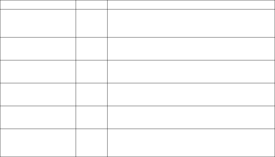
205

The kinetic model parameters that can be defined under “ParameterTable” are

listed in Table 7.1.

Table 7.1 Kinetic parameter models in sdb

Name

Unit

Description

Coordinate

N/A

Describe the geometry of dendrite for back diffusion model.

<Parameter name="coordinate" value="0" description =

"geometry of dendrite. 0 for plate; 1 for cylinder; 2 for

sphere" />

Interfacial_Energy

/Jm

Interfacial energy

<Parameter name="interfacial_energy" value="0.065"

description = "interfacial energy, unit = J/m^2"/>

Latent_heat

/Jm

Latent Heat of the alloy

<Parameter name="latent_heat" value="5.5e8" description =

"latent heat, unit=J/m^3"/>

Solute_Trapping_Parameter

N/A

Solute trapping parameter

<Parameter name="solute_trapping_parameter" value="1e-9"

description = "solute trapping parameter, unit=m"/>

Sound_velocity

N/A

Sound velocity

<Parameter name="sound_velocity" value="1000" description

= "sound velocity, unit=m/s"/>

Coarsening_Geometric_Factor

N/A

A factor adjusting adjust the coarsen speed of the dendrite.

<Parameter name="coarsening_geometric_factor" value="40"

description = "No unit"/>

206

7.2 Tutorial

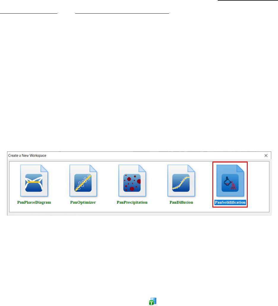
7.2.1 Step 1: Create a PanSolidification Project

Users can create a PanSolidification project through menu “File → Create a

New Workspace” or “File → Add a New Project” in an existing workspace. The

“Module Window” pops out for user to choose a module for the new project as

shown in

Figure 7.4. Choose “PanSolidification” module for Solidification simulation, and

the PanSolidification project will be created after user click on Create button or

double click on the PanSolidification icon.

Figure 7.4 Creating a PanSolidification workspace

7.2.2 Step 2: Load Thermodynamic and Mobility Database

The next step is to load the database, which is MgAlCaSn.tdb in this example.

Different from the normal thermodynamic database, this database also

contains mobility model parameters for the phases of interest in addition to the

thermodynamic model parameters. Both are needed for carrying out

solidification simulation. By clicking the button on the toolbar, a pop-up

window as shown in Figure 7.5 will open, allowing user to select the database

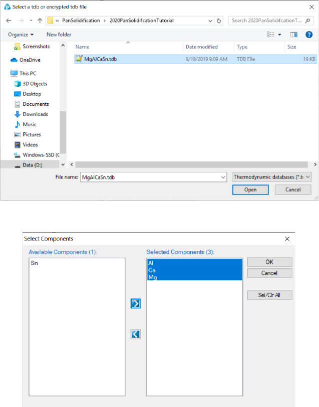
207

file. And Click “Open” to select the database, then a window as Figure 7.6 will

pop up for user to select components for PanSolidification simulation.

Figure 7.5 Dialog window for loading thermodynamic and mobility database.

Figure 7.6 Dialog window for components selection.

7.2.3 Step 3: Load Solidification Kinetic Database

A solidification kinetic database is required for solidification simulation. Such a

database contains kinetic parameters which are alloy dependent. To organize

these parameters in a more intuitive way, the standard XML format is adopted

and a set of well-formed tags are deliberately designed to define back diffusion

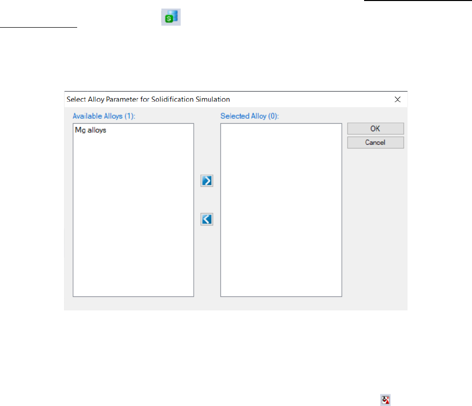
208

model for the morphology of primary phase (which could be plate, cylinder and

sphere) and its corresponding model parameters such as interfacial energy,

latent heat, coarsening geometric factor, dendrite tip factor, solute trapping

parameter, solid diffusivity factor and boundary layer factor.

In this example, the MgAlloys.sdb is prepared. To load a solidification

database, user should navigate the command through menu PanSolidification

→ Load SDB, or click icon from the toolbar. After MgAlloys.sdb is chosen,

a dialog box pops out automatically for user to select the alloy for the

simulation. As shown in Figure 7.7, Mg alloys is contained in this SDB file.

Figure 7.7 Dialog box for selecting alloy parameter.

7.2.4 Step 4: Solidification Simulation

Perform solidification simulation through menu bar PanSolidification -

>Solidification Simulation with Back Diffusion or click icon from the tool

bar. A dialog box entitled “Solidification Simulation with Back Diffusion”, as

shown in Figure 7.8, pops out for user’s inputs to set up the simulation

conditions: alloy composition and solidification conditions. When setting the

solidification conditions, users need to be careful about the units used for the

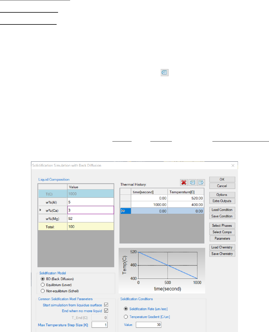
209

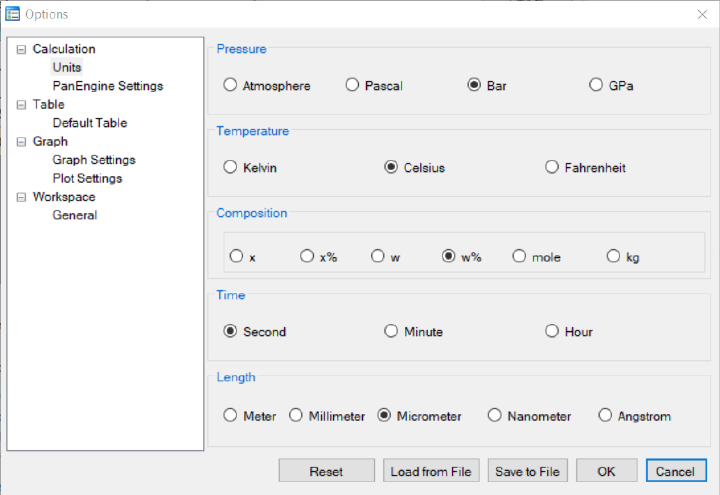
conditions. Click Option, a window as shown in Figure 7.9 will pops out for

units setting.

Alloy Composition: User can set alloy composition by typing in or use the

Load Chemistry function. User can also save the alloy composition through

Save Chemistry. This is especially useful when working on a multi-component

system, so that user does not need to type in the chemistry every time.

Solidification Conditions: The Cooling Rate of solidification can be defined

through Thermal History window. The cooling rate determined by cooling

curves can also be imported by click the icon as shown in Figure 7.8. The

Solidification Rate and Temperature Gradient can be defined from the

interface. As the Cooling Rate (CR), Solidification Rate (V) and Temperature

Gradient (G) has a relationship of CR = G*V, user may choose to provide either

Solidification Rate or Temperature Gradient.

User can also define the output Table and Graph within the Output Options

window.

210

Figure 7.8 Dialog box for setting solidification simulation conditions

Figure 7.9 Dialog box for setting units.

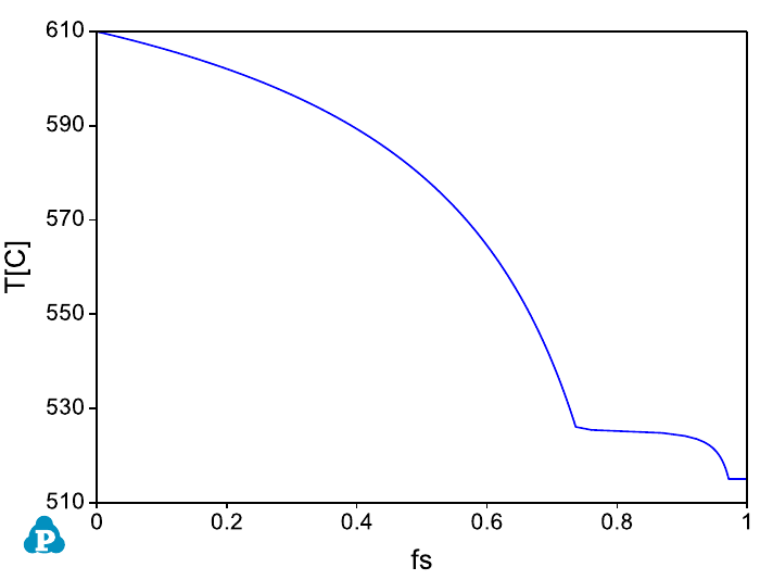
7.2.5 Step 5: Customize Simulation Results

As all other calculations available in Pandat

, upon the completion of the

solidification simulation, a default table with related solidification related

properties (time, temperature, secondary dendrite arm spacing, solid and liquid

phase fractions, etc.) is automatically generated and a default graph for

temperature (T) vs solid fraction (fs) is displayed as shown in Figure 7.10. User

can refer to sections 2.3 and 2.4 to learn how to customize simulated graph

and table.

211

Figure 7.10 Default graph plotting Temperature vs f

during solidification.