212
8 Property
Property calculation has been added into Pandat
TM
and is characterized in
three categories, thermodynamic property, physical property and kinetic
property. The database format and the equations for these properties are
described below.
8.1 Thermodynamic Property
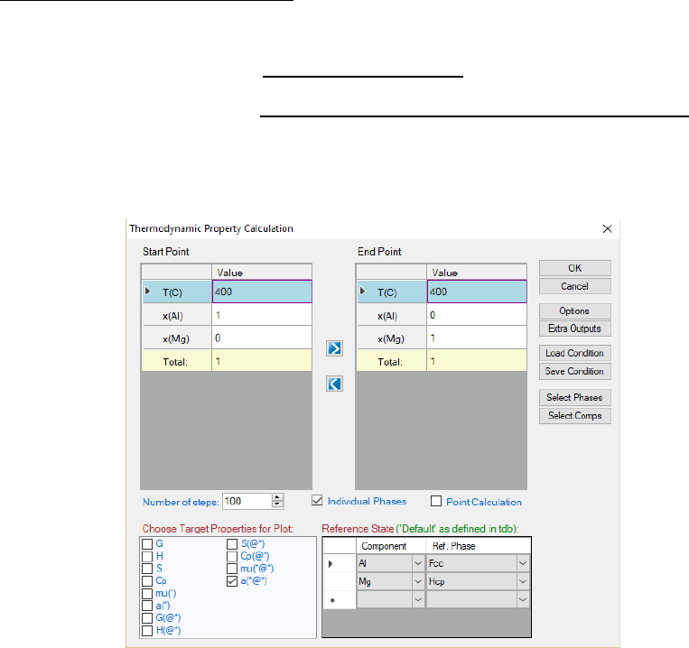
The Thermodynamic Property function is used to calculate thermodynamic
properties, such as Gibbs energy, enthalpy, entropy, chemical potential,
activity, etc. It is under the PanPhaseDiagram module. User can access this
function through the menu (Property → Thermodynamic Property) after the
thermodynamic database is loaded. A popup window will allow user to input
calculation conditions as shown in Figure 8.1.
Figure 8.1 Thermodynamic Property calculation dialog
The calculation is set as a line calculation with the desired thermodynamic
properties output. User may select the thermodynamic properties as needed by
213
checking the boxes in front of each property as shown in Figure 8.1 and specify
the reference state for each element. The selected property will be calculated
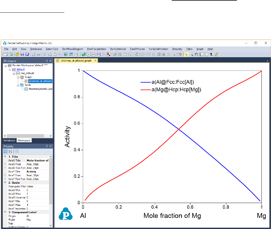
and graph plotted as shown in Figure 8.2. If two or more thermodynamic
properties are selected, they will be plotted separately. Experienced user can
also get these results directly from the Line Calculation in the
PanPhaseDiagram module with proper syntax using self-defined table.
Figure 8.2 Thermodynamic Property calculation results

214
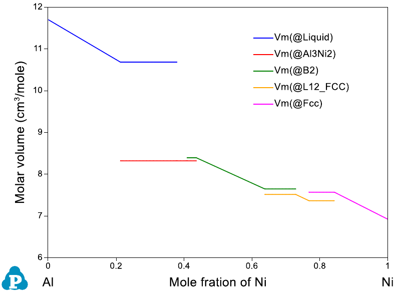
8.2 Physical Property
Physical property calculation implemented in Pandat
TM
allows user to calculate
the molar weight, molar volume, density, surface tension and viscosity. The
interface is similar to the Thermodynamic property calculation as shown in
Figure 8.3. User can set up the calculation condition as a line calculation and
select the properties to be calculated. The default graph is the calculated
property as shown in Figure 8.4 as an example. Again, if two or more
properties are selected, all of them will be plotted one by one.
The detailed calculation method for each property and the format of the
database file are described in the following sections.
Figure 8.3 Physical property calculation dialog
215
Figure 8.4 Physical property calculation results
8.2.1 Molar Weight and Phase Weight Fraction
The molar weight for a phase is calculated from the atomic weights of the
elements involved in the phase. The unit is kg/mol-atoms. Since atomic
weights of elements have been included in Pandat, no input is required in the
database TDB file.
For example, an Fcc phase in Al-Cu binary system with
0.9
Al
x =
and
0.1
Cu
x =
,
its molecular weight is
-3 -3
0.9 26.982 10 0.1 63.546 10
fcc
Al Al Cu Cu
MW x M x M= + = +
-3
30.6384 10 ( / )kg mol atoms= −
(8.1)
8.2.2 Molar Volume and Phase Volume Fraction
The molar volume can be calculated by Pandat
TM
if the model parameters are
properly defined in the database file. The molar volume of a pure component is
described as a function of temperature and pressure, and the excess molar
216
volume of a phase is described in the format similar to that of excess Gibbs
energy. The unit of molar volume is
3
/m mol atoms−
. In the database (.TDB) file,
the format of molar volume is:
PARAMETER Vm(Fcc,Al;0) 298.15 +9.7743e-006*exp(6.91213e-005*T+1.62267e-
011*T**3+0.413484*T**(-1)); 3000 N !
PARAMETER Vm(Fcc,Fe;0) 298.15 +6.72092e-006*exp(6.97895e-005*T); 3000 N !
PARAMETER Vm(Fcc,Al,Fe:Va;0) 298.15 -3e-6; 3000 N !
The calculation of molar volume for a phase is
()
i ij
ok
m i m i j m i j
V xV x x V x x= + −
(8.2)
where
ij
m
V
is the parameter for the excess molar volume of this phase.
Molar volume of a system with phase mixture is calculated by
mm
V f V
=
(8.3)
where
f
and
m
V
are the molar fraction and molar volume for phase
.
Note that, if a phase is described by a compound-energy-formalism (CEF) with
multi-sublattices, the molar volume is automatically described as a function of
T, P, and site fraction (y) following the format of the Gibbs energy. This will
introduce many end members in the molar volume and may lead to instability
in the calculated molar volume. In reality, molar volume should be a function
of mole fraction (x) instead of site fraction (y), it is thus recommended to define
the molar volume of a phase separately from its Gibbs energy if the phase is
described by the CEF model. This can be realized through the user-defined
molar volume property (section 3.3.8).
Using the Al-Ni binary system as an example, type “VARIABLE_X” is defined as
property “V
m
”:
Type_Definition v GES AMEND_PHASE_DESCRIPTION * VARIABLE_X Vm !

217
which means any phase with the Type_Definetion “v” will use mole fractions as
the variables of Vm. Here are examples to define the molar volume parameters
for the Liquid and L12_FCC phases:
Phase Liquid %v 1 1 !
Parameter Vm(Liquid,Al;0) 298.15 +V_Al_Liquid; 3000 N !
Parameter Vm(Liquid,Ni;0) 298.15 +V_Ni_liquid; 3000 N !
Phase L12_FCC %v 2 0.75 0.25 !
Parameter Vm(L12_FCC,Al;0) 298.15 +0.935*V_Al_fcc; 3000 N !
Parameter Vm(L12_FCC,Ni;0) 298.15 +0.935*V_Ni_fcc; 3000 N !
In this case, the molar volume of L12_FCC is calculated as:
0.935* * 0.935* *
fcc fcc
m Al Al Ni Ni
V x V x V=+
(8.4)
although the L12_FCC phase is described by CEF model with two sublattices.
Please refer to the example #28 in the example book for detail information.
8.2.3 Density
Density is calculated from molar volume and the molar weight. It requires the
molar volume parameters in database. The unit for density is
3
/kg m
. Density of
a phase is defined as
(8.5)
The density of a system with phase mixture is calculated from the molar weight
and the molar volume of the mixture:
(8.6)

218
8.2.4 Viscosity
A function to calculate viscosity of liquid phase is added into current Pandat
TM
.
The model used for describing the viscosity of liquid phase is semi-empirical
relation presented in the paper by Seetharaman and Du [1994See],
=
RT
G
A
*
exp
(8.7)
with
V
hN
A =
(8.8)
where V is the molar volume of the melt, h the Plank’s constant, N the
Avogadro’s number.
*
G
is the Gibbs energy of activation, and can be
calculated by
++=
jimix
mo
ii
xxRTGGxG 3
*
(8.9)
where x
i
and x
j
are the molar fractions of component i and j,
o
i
G
, Gibbs energy
of activation of component i, and
mix
m
G
, Gibbs energy of mixing. The
calculation of molar volume is given in above sections. The parameter for the
activation energy of a pure component in database TDB file has the format
Parameter ActivationEnergy(Liquid,Al;0) 298.15 15051+13.519*T; 2000 N !
8.2.5 Surface Tension
Current Pandat has another new function to calculate surface tension of liquid
phase. The model for calculating surface tension of liquid is the semi-empirical
relationship proposed by Yeum et al. [1989Yeu] to estimate the surface
tensions of binary alloys based on the model of Butler [1932But].
i
i
i
i
a
a
S
RT
,
ln+=
(8.10)
where
i
,
,
i
a
and
i
a
are the surface tension, activity at the surface and activity in
the bulk of component i. And
i
S
is the surface monolayer area,
219
3/23/1
ii
VbNS =
(8.11)
where b is geometric factor, N the Avogadro’s number, and V
i
molar volume of
component i. This approach was extended to calculate surface tensions of
multicomponent liquid alloys [1997Zha]. The calculation of molar volume is the
same as given in section 8.2.2. The ratio of the coordination number for the
surface atoms to that for the atoms in the bulk phase, b, is represented by a
parameter beta, described in database (.tdb) file in the format as
Parameter Beta(Liquid,Al;0) 298.15 0.83; 2000 N !
220
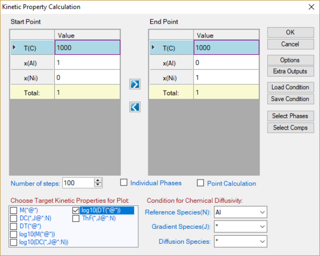
8.3 Kinetic Property
Diffusivity related properties can be calculated from Pandat
TM
as long as the
corresponding species mobility parameters are available in the database. User
can input the calculation condition through the interface shown in Figure 8.5
and select the desired properties for output. The default graph is the selected
property as shown in Figure 8.6. If two or more properties are selected, they
will be plotted separately.
Details on the kinetic models for the multicomponent diffusion are referred to
the literature [1982Ågr, 1992And]. Only the key equations related to the
properties of mobility, tracer diffusivity and chemical diffusivity are given in the
below sections.
Figure 8.5 Kinetic Property calculation dialog
221
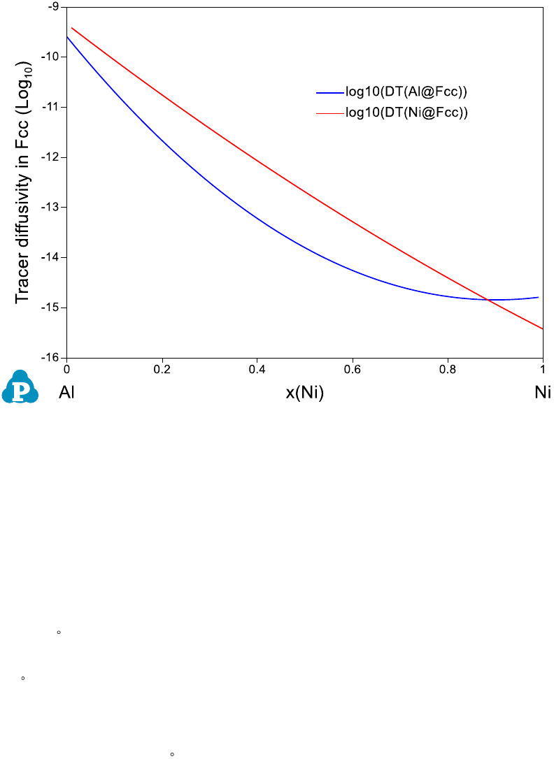
Figure 8.6 Calculated diffusivity in the Al-Ni system
8.3.1 Atomic Mobility
In order to simulate diffusivity related properties such as chemical diffusivities
of components, atomic mobility data of species in phases are required and
stored in the database. Mobility of species k is related to its activation energy
(
k
Q
) by
/
k
Q RT
kk
M M e
−
=
(8.12)
where
k
M
is a frequency factor, R is the gas constant and T the temperature in
Kelvin. Define
k
MQ
as
ln ln
k k k k
MQ RT M RT M Q= = −
(8.13)
Then, atomic mobility can be calculated from
k
MQ
.
k
MQ
is a function of
composition, temperature and pressure and can be expressed as Redlich-Kister
type of polynomial expansion as for the excess Gibbs energy [1982Ågr]. Each
polynomial coefficient is stored in database. For example, the coefficient for

222
term contributed to Al from Ni in Fcc phase (
,Ni
Al
MQ
) is described in TDB file as
follows,
Parameter MQ(Fcc&Al,Ni;0) 298.15 -285517+R*T*Ln(0.0007933); 6000 N !
In Pandat, atomic mobility of species can be obtained through table operation
with field of “M(*@*)”. For example, M(Al@Fcc) represents the atomic mobility
of Al in Fcc phase.
8.3.2 Tracer Diffusivity
Tracer diffusivity of a species k is directly related to its atomic mobility by
*
kk
D RTM=
(8.14)
where R is the gas constant and T the temperature. Tracer diffusivity can be
obtained in Pandat
TM
from table with field of “DT(*@*)”. For example, the tracer
diffusivity of Al in Fcc can be extracted from calculation result with the table
field of “DT(Al@Fcc)”. The natural logarithm of the tracer diffusivity is available
with “logDT(*@*)”.
8.3.3 Chemical Diffusivity
Chemical diffusivity of species k,
n
kj
D
, could be calculated by
n
kj kj kn
D D D=−
(when j is substitutional) (8.15)
n
kj kj
DD=
(when j is interstitial) (8.16)
and
()
ii
kj ik k i i ik i Va i
jj
i S i S
D u u M u y M
uu
= − +
(8.17)
where S represents the set of the substitutional species,
ik
.is the Kronecker
delta, and
i
is the chemical potential of species i.
k
u
is defined as

223
k
k
j
iS
x
u
x
=
(8.18)
Chemical diffusivity of species k in phase p can be obtained in Pandat
TM
with
the table field of “DC(k,j@p:n)”, where j and n are the gradient species and the
reference species, respectively. Its corresponding natural logarithm is
“logDC(k,j@p:n)”.
8.4 User defined properties
Pandat allows user to define any property of a phase or a system following
some simple syntax rules. The user-defined-property database can be added
to the original database, either TDB or PDB files, through Append database
function. (Please refer to Section 3.3.9 for the detailed description on Append
database function). Users can also add the user-defined-property parameters
into their home-developed TDB files to develop a combined database for User-
defined property calculations.
Three methods are implemented in Pandat to add User-defined-properties,
depending on the nature of the properties. Key words Phase_Property;
System_Property and Property are used in the syntax respectively.
Phase Property is used to define a property of a phase with a similar
expression which describes the Gibbs energy of a disordered solution phase.
Let U be the user-defined phase property and it is expressed as:
1
1 1 1
()
c c c
o k k
i i i j i j ij
i i j i k
U xU x x x x L
−
= = = +
= + −
(8.19)
where
i
x
is the molar fraction of component i and
0
i
U
is the property of the
pure component i,
k
ij
L
is the k
th
order interaction parameter between
components i and j. The syntax used in the TDB file are:
Type_Definition z PHASE_PROPERTY U 1 !
Type_Definition v GES AMEND_PHASE_DESCRIPTION * VARIABLE_X U !
224
In this definition, “v” is the identifier, “*” means any phase, and VARIABLE_X is
the key word indicating X as the variable. The meaning of this definition is that
any phase with the identifier “v” will use mole fractions (x) as the variables for
property U.
System Property is used to define a property of a system with more than one
phase. For a property in a system with multi-phase mixture, the property of the
system is the weighted average of that of each phase. By default, the arithmetic
mean is applied to a user defined Phase Property in a multi-phase system. For
example, the user defines Phase Property U in a system with and β two-
phase mixture. The property of U of this system is calculated by
U f U f U
=+
(8.20)
If the simple arithmetic mean does not apply, more complicated expression can
be defined by User through Command System Property. For example, the
value of the system property can be calculated through the function:
0
()
i
i
i
U f U f U f f M f f
+
=
= + − −
(8.21)
where
U
+
is the user defined property of U in α+β two phase region.
U
and
U
is the property U in α and β phase respectively; f
α
and f
β
are the phase
fraction of α and β phase respectively. M
i
are the i
th
order of the additional
parameters which are used to describe additional effects on the user defined
property U.
The syntax for the System Property used in the TDB file is:
System_Property Sys_U 1 !
Parameter L(Sys_U, Alpha, Beta;0) 298.15 M0; 3000 N !
Parameter L(Sys_U, Alpha, Beta;1) 298.15 M1; 3000 N !
Using command Property, user can also define special properties associated
with phases in the original database. Any phase property available from Pandat
225
Table can be used for user-defined property, such as G, H, mu, and ThF.
However, the star symbol in a property, like mu(*), cannot be used.
The syntax for the Property used in the TDB file is:
Property GFcc_GLiq 298.15 G(@Fcc)-G(@Liquid); 6000 N !
8.4.1 User-defined Molar Volume Database
The molar volume (V
m
) is one of the pre-defined properties in Pandat. The
molar volume of a pure component is described as a function of temperature
and pressure, and the excess molar volume of a phase is usually described in
the format similar to that used to describe the excess Gibbs energy of the
phase. Note that, if a phase is described by a compound-energy-formalism
(CEF) with multi-sublattices, the molar volume is automatically described as a
function of T, P, and site fraction (y) following the format of the Gibbs energy.
This will introduce many end members in the molar volume and may lead to
incontinuity in the calculated molar volume. In reality, molar volume should be
a function of mole fraction (x) instead of site fraction (y), it is thus
recommended to define the molar volume of a phase separately from its Gibbs
energy if the phase is described by the CEF model. This can be realized
through the user-defined molar volume property.
In brief, the molar volume of element i with crystal structure φ can be
expressed as:
0
0
( ) exp( 3 )
T
i
T
V T V dT
=
(8.22)
where V
0
is the molar volume under atmospheric pressure at the reference
temperature T
0
. And is the coefficient of linear thermal expansion (CLE). The
volume of a phase with crystal structure φ can then be obtained via the
Redlich-Kister polynomial:
()
ex
i i m
i
V T xV V
=+
(8.23)

226
where x
i
is the mole fraction of element i and
ex
m
V
is the excess molar volume.
Using ternary system as an example, the
ex
m
V
can be expressed by:
1
,,
11
()
cc
ex k k
m i j i j ij i j p i j p
i j i k
V x x x x L x x x L
−
= = +
= − +
(8.24)
The terms
,
k
ij
L
and
,,i j k
L
are the interaction parameters from the constituent
binary and the ternary systems, respectively. The standard unit of molar
volume is m
3
/mol.atom.
The molar volume database also enables us to calculate the density based on
the relationship of
m
M
V
=
(ρ is the mass density, M is the molar mass, and
V
m
is the molar volume).
Here we use the Al-Ni binary system as an example to demonstrate the
calculation of molar volume through user-defined property. Please refer to the
AlNi_Vm.tdb for details. In the beginning of the database file, a Type_Definition
is given as below:
Type_Definition v GES AMEND_PHASE_DESCRIPTION * VARIABLE_X Vm !
In this definition, “v” is the identifier, “*” means any phase, and VARIABLE_X is
the key word indicating X as the variable. The meaning of this definition is that
any phase with the identifier “v” will use mole fractions (x) as the variables for
V
m
. Here are examples to define the molar volume parameters for the Fcc and
L12_FCC phases in the Al-Ni system:
Phase Fcc %(v 1 1 !
Constituent Fcc: Al,Ni:!
Parameter Vm(Fcc,Al;0) 298.15 +V_Al_fcc; 3000 N !
Parameter Vm(Fcc,Ni;0) 298.15 +V_Ni_fcc; 3000 N !
Parameter Vm(Fcc,Al,Ni;0) 298.15 -2.85e-6; 3000 N !
Phase L12_FCC %v 2 0.75 0.25 !
227
Constituent L12_FCC: Al,Ni:Al,Ni:!
Parameter Vm(L12_FCC,Al;0) 298.15 +V_Al_fcc; 3000 N !
Parameter Vm(L12_FCC,Ni;0) 298.15 +V_Ni_fcc; 3000 N !
Parameter Vm(L12_FCC,Al,Ni;0) 298.15 -3.2e-6; 3000 N !
Even though the L12_FCC phase is modeled by CEF model with two sublattices,
four end members, and 13 interaction parameters, its molar volume property
can be described as a function of
like a solution phase through user-defined
property. In other words, the molar volume of L12_Fcc is:
(8.25)
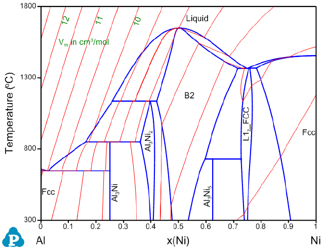
Figure 8.7 shows the calculated Al-Ni binary phase diagram with molar volume
contour lines. Please refer to AlNi_Vm.pbfx and section 3.3.5 for details on the
calculation of contour diagrams.
Figure 8.7 Al-Ni binary phase diagram with the calculated contour lines of
molar volume (cm
3
/mol).
228
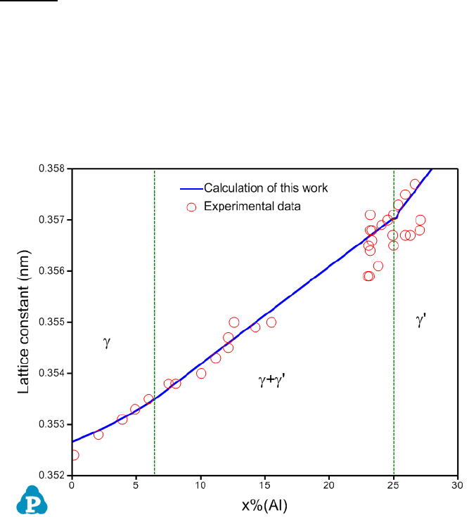
The lattice constant, or lattice parameter, refers to the physical dimension of
unit cells in a crystal lattice. For FCC crystal structure, the lattice constant can
be calculated by:
(8.26)
An example is given for the calculation of lattice constant in Ni-Al binary at Ni-
rich corner. The calculated lattice constant agrees with the experimental data
well as is shown in Figure 8.8. Please refer to AlNi_lattice.pbfx for details. It
should point out that the unit of Vm in the above equation is cm
3
/mol.
Figure 8.8 Comparison of calculated and measured lattice constants of the γ
and γ’ phases in Ni-Al binary alloys at room temperature
8.4.2 Thermal Resistivity and Thermal Conductivity
Thermal conductivity of a pure element or a stoichiometric phase at
temperature above 273 K is described as a function of temperature using the
following equation:
12
A BT CT DT
−
= + + +
(8.27)
229
where κ is the thermal conductivity and T is the temperature in Kelvin. This
function can reasonably fit most of the experimental thermal conductivity data
of elements at temperature above 273 K.
The thermal conductivity of solid solution phase can be calculated from
thermal resistivity, which is the reciprocal of thermal conductivity. According
to the Nordheim rule, the thermal resistivity (ρ) of a solid solution phase can be
described by the following Redich–Kister polynomials:
0
()
i
AB A A B B A B i A B
i
x x x x L x x
=
= + + −
(8.28)
where
AB
is the thermal resistivity of the solution phase in the A-B system.
x
j
and ρ
j
are the mole fraction and thermal resistivity of pure elements j,
respectively. L
i
are the i
th
order interaction parameters which are used to
describe the effect of solute elements on the thermal resistivity. In general, the
interaction parameter can be expressed as:
1
i i i i
L a bT cT
−
= + +
(8.29)
where the parameters a
i
, b
i
and c
i
are evaluated based on the experimental
data.
The interface scattering parameters is introduced to describe the effect of the
second phase on the thermal resistivity in two-phase region. The thermal
resistivity of the two-phase region is described as following:
0
()
i
i
i
f f f f M f f
+
=
= + − −
(8.30)
where ρ
α+β
is the thermal resistivity of the alloys in α+β two-phase region, f
p
and
ρ
p
(p = α, β) are the mole fraction and thermal resistivity of the phase p,
respectively. M
i
, which can be considered to be linearly temperature dependent,
is the i
th
interface scattering parameter and and can be evaluated from the
experimental data. The thermal conductivity of alloy system and the value of
each phase can be obtained by using the reciprocal of the thermal resistivity
values through output option.
230
In this example, thermal resistivity of the Al-Mg binary alloys is described
using the user-defined property function.
As shown in the AlMg_ThRss.tdb, the thermal resistivity ThRss property is first
defined as user-defined property since it hasn’t been pre-defined in the current
Pandat software.
Type_Definition z PHASE_PROPERTY ThRss 1 !
In accordance, the following definition is also needed to add this property to the
original database.
Type_Definition e GES AMEND_PHASE_DESCRIPTION * VARIABLE_X ThCond !
As is seen, the thermal resistivity of the Fcc phase or the Hcp phase follows the
same format as that of Gibbs energy for a disordered solution phase.
Parameter ThRss(Liquid,Al;0) 298.15 1/ThCond_Al_Liq; 3000 N !
Parameter ThRss(Liquid,Mg;0) 298.15 1/ThCond_Mg_Liq; 3000 N !
Parameter ThRss(Fcc,Al;0) 298.15 1/ThCond_Al_Fcc; 3000 N !
Parameter ThRss(Fcc,Mg;0) 298.15 1/ThCond_Mg_Hcp; 3000 N !
Parameter ThRss(Fcc,Al,Mg;0) 298.15 0.02566-1.3333e-05*T+14.5*T^(-1);
3000 N !
Parameter ThRss(Hcp,Al;0) 298.15 1/ThCond_Al_Fcc; 3000 N !
Parameter ThRss(Hcp,Mg;0) 298.15 1/ThCond_Mg_Hcp; 3000 N !
Parameter ThRss(Hcp,Al,Mg;0) 298.15 0.02140-1.3669e-05*T+12.7158*T^(-1);
3000 N !
Parameter ThRss(Hcp,Al,Mg;1) 298.15 0; 3000 N !
Parameter ThRss(Hcp,Al,Mg;2) 298.15 0.14825-7.7706e-05*T+25.3031*T^(-1);
3000 N !
Thermal resistivity of the intermetallic phases with narrow solid solubility rage
in the phase diagrams is treated like that of a stoichiometric compound phase,
i.e., it is composition independent and is described as below:
231
Parameter ThRss(AlMg_Beta,*;0) 298.15 1/42; 6000 N !
Parameter ThRss(AlMg_Eps,*;0) 298.15 1/42; 6000 N !
Parameter ThRss(AlMg_Gamma,*;0) 298.15 -0.03267+2.7412e-05*T+20.722*T^(-1);
6000 N !
In order to describe the thermal resistivity within two-phase region, a system
property, Sys_ThRss, is then defined by the command:
System_Property Sys_ThRss 1 !
Parameter L(Sys_ThRss, Fcc, AlMg_Beta;0) 298.15 0.005; 3000 N !
Parameter L(Sys_ThRss, Hcp, AlMg_Gamma;0) 298.15 0; 3000 N !
Parameter L(Sys_ThRss, Hcp, AlMg_Gamma;1) 298.15 0.01; 3000 N !
After the thermal resistivity has been properly modeled for each phase, the
thermal conductivity of each phase and that of the system can be directly
calculated and outputed by using extra output in Pandat defined as
1/ThRss(@*) and 1/Sys_ThRss, respectively. The comparisons between the
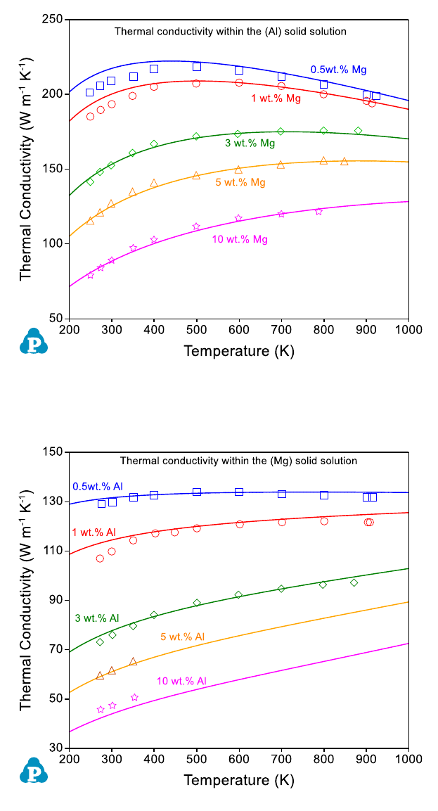
calculated and measured thermal conductivities of the Al-Mg alloys are shown
in Figure 8.9 to Figure 8.11. This example demonstrates that the user-defined
property function is very powerful and flexible to allow users define various
types of properties. The property can be a function of any phase properties that
can be calculated by PanPhaseDiagram module.
232
Figure 8.9 Comparison between the calculated and measured thermal
conductivities in the (Al) solid solution in the Al-Mg binary system
Figure 8.10 Comparison of the calculated and measured thermal conductivities
in the (Mg) solid solution in the Al-Mg binary system
233
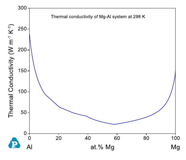
Figure 8.11 Calculated thermal conductivities of Mg-Al system at 298 K.
8.4.3 Calculation of T
0
Curve Using User-defined Property
T
0
curve is the trace of a series of points in a two-phase field at which the
Gibbs energy of the two phases are identical. In this example, the original
database is ABC.tdb, and the T
0
-curve property is defined in the Appended
database ABC_T0.tdb. In the ABC_T0.tdb file, the T
0
-curves of Bcc/Liquid and
Fcc/Liquid phases are defined as:
Property GFcc_GLiq 298.15 G(@Fcc)-G(@Liquid); 6000 N !
Property GBcc_GLiq 298.15 G(@Bcc)-G(@Liquid); 6000 N !
Where “Property” is the key word for user-defined property and G(@Bcc),
G(@Fcc), G(Liquid) are the Gibbs free energies of the Bcc, Fcc, and Liquid
phases, respectively. Note that, the Bcc, Fcc and Liquid are defined in the
ABC.tdb. In this particular case, the above “Property” can be directly defined in
the ABC.tdb, i.e., the ABC.tdb and ABC_T0.tdb can be combined into one
database. This example demonstrates that user-defined property can be
234
separated from the original database. This design makes it possible to obtain
user-defined properties even the original database is in encrypted pdb format.
In this example, the GBcc_GLiq property is defined as the Gibbs free energy
difference between the Bcc phase and the Liquid phase, and GFcc_GLiq
property is defined as the Gibbs free energy difference between the Fcc phase
and the Liquid phase.
Using the Contour function (Section 3.3.5), we can calculate contour maps of
these user-defined properties and plot them on the calculated phase diagram.
When we set the calculation condition as GBcc_GLiq=0, the T
0
curve for
Bcc/Liquid is obtained as is shown by the green line in Figure 8.12. Similarly,
by setting GFcc_GLiq=0, we obtain the T
0
curve for Fcc/Liquid as is shown by
the red line in Figure 8.12.
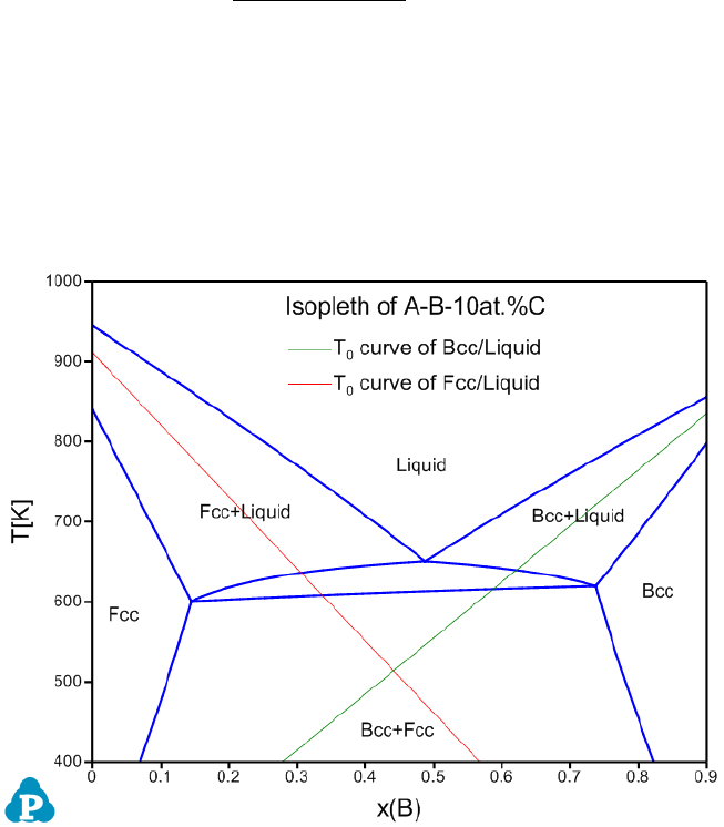
Figure 8.12 Calculated isopleth of A-B-10at.%C with T
0
curves of Bcc/Liquid
and Fcc/Liquid phases
User can run the ABC_T0.pbfx batch file to obtain Figure 8.12. Two points
should be addressed for this batch file:
235
• Both the “start” and “stop” values should set to be zero for the contour
mapping as following to get the T
0
line.
<contour name="Contour_T0_Fcc_Liq" property="GFcc_GLiq" start ="0" stop ="0"
step="1"/>
<contour name="Contour_T0_BCC_Liq" property="GBcc_GLiq" start ="0" stop ="0"
step="1"/>
• To obtain the T
0
curve, each phase needs to be considered individually, thus
the equilibrium type is set to be “individual”
<individual_phase value="true"/>
<equilibrium_type type="individual"/>
8.4.4 Calculation of Spinodal Curve Using User-defined
Property
A Spinodal curve is where the determinant of the Hessian of Gibbs free energy
with respect to composition is zero. For a phase with c-components, above
condition is expressed as
=0 (8.31)
where the molar fraction of component 1 is chosen as the dependent variable.
The second derivative of G w.r.t. molar fractions can be calculated from the
thermodynamic factors:
(j,k=2,3,…,c) (8.32)
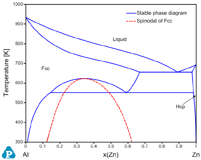
Example #1: Spinodal curve of Fcc phase in the Al-Zn binary system
In this example, the spinodal curve of the Fcc phase in the Al-Zn binary system
is calculated through user-defined property. A user-defined property d2GdxZn2
for the Fcc phase is defined in AlZn_Spinodal.tdb as:
236
Property d2GdxZn2 298.15 ThF(Zn,Zn@Fcc)-ThF(Al,Zn@Fcc)-ThF(Zn,Al@Fcc)+
ThF(Al,Al@Fcc); 6000 N !
where ThF(Zn,Zn@Fcc), ThF(Al,Zn@Fcc), ThF(Zn,Al@Fcc), and ThF(Al,Al@Fcc)
are the thermodynamic factors of Fcc phase. Since the value of d2GdxZn2 is
usually a large number, we define the Hessian function, HSN, as d2GdxZn2
multiplied by a factor 1E-4:
Property HSN 298.15 1e-4*d2GdxZn2; 6000 N !
As shown in the AlZn_Spinodal.pbfx, the AlZn_Spinodal.tdb is appended to the
AlMgZn.tdb. The spinodal line is calculated through contour mapping by using
following conditions:
<contour name="Spinodal" property="HSN" start="0" stop="0" step="1"/>
<equilibrium_type type="individual"/>
The calculated Fcc Spinodal is shown in Figure 8.13 with the stable Al-Zn
binary phase diagram.
Figure 8.13 Calculated spinodal curve of the Fcc phase within the Al-Zn binary
system
237
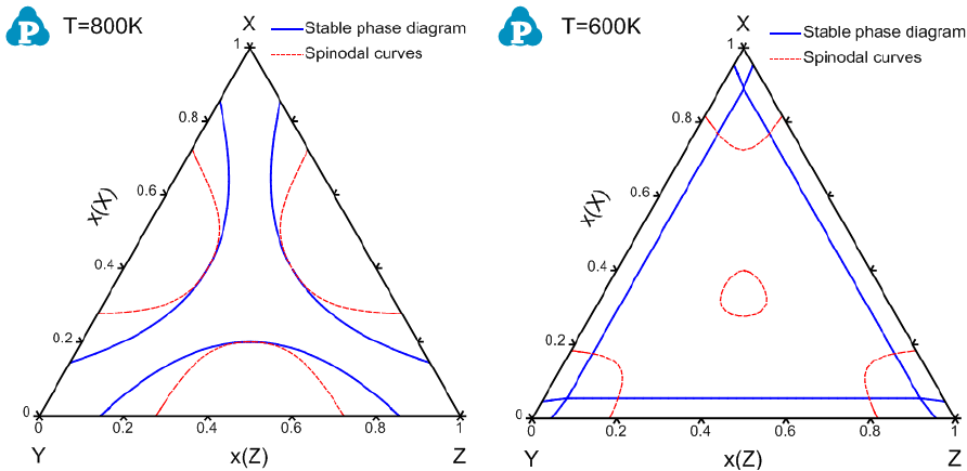
Example #2: Spinodal curve of Fcc phase in the X-Y-Z ternary system
In this example, the original database is XYZ.tdb, and the user-defined HSN
property is defined in XYZ_Spinodal.tdb as described below:
Property d2Gdx2 298.15 ThF(Y,Y@Fcc)-ThF(X,Y@Fcc)-ThF(Y,X@Fcc)+ThF(X,X@Fcc);
6000 N !
Property d2Gdy2 298.15 ThF(Z,Z@Fcc)-ThF(X,Z@Fcc)-ThF(Z,X@Fcc)+ThF(X,X@Fcc);
6000 N !
Property d2Gdxy 298.15 ThF(Y,Z@Fcc)-ThF(X,Z@Fcc)-ThF(Y,X@Fcc)+ThF(X,X@Fcc);
6000 N !
Property HSN 298.15 1e-10*(d2Gdx2 * d2Gdy2 - d2Gdxy * d2Gdxy); 6000 N !
Note that the HSN property within the XYZ ternary system is derived and
described as a function of the thermodynamic factor ThF. A factor of 1E-10 is
used to scale the HSN property since the numerical value of HSN is very big.
Again the spinodal lines are calculated through contour mapping. Details can
be found in XYZ_Isotherm_Spinodal.pbfx and XYZ_Isopleth_Spinodal.pbfx.
Figure 8.14 and Figure 8.15 show the calculated spinodal curves superimposed
on the stable phase diagrams:
Figure 8.14 Calculated isothermal sections of the X-Y-Z system at 800 and
600K with spinodal curves, respectively
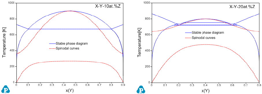
238
Figure 8.15 Calculated isopleths within the X-Y-Z system for 10 and 20 at.%Z
with spinodal curves, respectively